
Tokens & Attention: The Engine of Modern Sequence Modeling
Tokens & Attention: The Engine of Modern Sequence Modeling
In Chapter 6: Normalization & Regularization, we stabilized deep neural activations.
Now we tackle sequential data: natural language, audio, and code.
For decades, sequential data was processed by Recurrent Neural Networks (RNNs and LSTMs). However, RNNs process tokens one by one ($t=1, 2, 3, \dots$). This sequential bottleneck prevents parallelization across GPU cores and makes remembering information from 1,000 tokens ago mathematically treacherous.
In 2017, Vaswani et al. introduced the Transformer, replacing recurrence with Self-Attention.
This chapter explains how text turns into tokens, how token embeddings construct vector spaces, and how Query-Key-Value attention routes information dynamically across sequences.
1. Core Intuition: The Filing Cabinet & Search Engine
Imagine entering a massive university library with a specific question: "What is the capital of France?"
'Looking for capital of France'"] --> Match["Dot Product Compatibility: Q · Kᵀ"] subgraph Keys["Filing Cabinet (Keys K)"] K1["Key K1: 'Geology of Mars' (Score: 0.01)"] K2["Key K2: 'French Geography & Paris' (Score: 0.95)"] K3["Key K3: 'Python Programming' (Score: 0.04)"] end Keys --> Match Match --> SM["Softmax Normalization
Weights A = [0.01, 0.95, 0.04]"] SM --> Val["Weighted Extraction over Values (A · V)"] Val --> Out["Context Output: 'Paris is the capital of France'"]
In Self-Attention: - Query ($Q$): What each token is currently searching for. - Key ($K$): What each token advertises about its contents. - Value ($V$): The actual semantic information the token transfers if a match occurs.
Every word simultaneously asks questions of every other word in the sentence, weighting and aggregating relevant context in a single parallel operation.
2. From Text to Continuous Vectors: Tokenization & Embeddings
A GPU cannot perform arithmetic on ASCII text strings like "deep learning". Text must be mapped into continuous floating-point vectors.
Byte-Pair Encoding (BPE)
Modern language models do not split text by entire words (which produces millions of rare words) or individual characters (which creates excessively long sequences).
They use Byte-Pair Encoding (BPE):
1. Start with raw byte vocabulary (256 base characters).
2. Scan a large corpus and count the most frequent adjacent pairs of bytes.
3. Iteratively merge the top pairs into new subword tokens (e.g. "trans" + "former" $\to$ "transformer").
4. Any unknown word can be broken down into subword fragments or individual bytes, ensuring zero out-of-vocabulary failures.
The Embedding Table
Once text is tokenized into integer IDs $\mathbf{t} = [142, 8931, 25]$, each integer indexes a row in an Embedding Matrix $\mathbf{E} \in \mathbb{R}^{V \times D_{model}}$:
$$\mathbf{x}_i = \text{Embedding}(\mathbf{t}_i) = \mathbf{E}_{\mathbf{t}_i, :}$$
Where $V$ is vocabulary size (typically 32,000 to 128,000) and $D_{model}$ is the hidden representation dimension (typically 2,048 to 8,192).
3. Scaled Dot-Product Attention: Mathematical Derivation
Given a sequence of $S$ input token vectors $\mathbf{X} \in \mathbb{R}^{S \times D_{model}}$, we project them into three separate spaces using learned weight matrices $\mathbf{W}_Q, \mathbf{W}_K, \mathbf{W}_V \in \mathbb{R}^{D_{model} \times d_k}$:
$$\mathbf{Q} = \mathbf{X}\mathbf{W}_Q, \quad \mathbf{K} = \mathbf{X}\mathbf{W}_K, \quad \mathbf{V} = \mathbf{X}\mathbf{W}_V$$
Zero Hidden Premises: Symbol Breakdown
| Symbol | Mathematical Domain | OpenCL Hardware & Memory Mapping |
|---|---|---|
| $S$ | $\mathbb{N}^+$ | Context sequence length (e.g. 2,048 or 4,096 tokens) |
| $D_{model}$ | $\mathbb{N}^+$ | Model hidden representation dimension (e.g. 4,096 in LLaMA-7B) |
| $H$ | $\mathbb{N}^+$ | Number of parallel attention heads (e.g. 32 heads) |
| $d_k$ | $\mathbb{N}^+$ | Per-head projection dimension ($d_k = D_{model} / H$, e.g. 128) |
| $\mathbf{X}$ | $\mathbb{R}^{S \times D_{model}}$ | Input activation buffer in GPU VRAM ($S \times D_{model} \times 4$ bytes) |
| $\mathbf{W}_Q, \mathbf{W}_K, \mathbf{W}_V$ | $\mathbb{R}^{D_{model} \times d_k}$ | Query, Key, and Value projection weight matrices |
| $\mathbf{Q}, \mathbf{K}, \mathbf{V}$ | $\mathbb{R}^{S \times d_k}$ | Projected Query, Key, and Value activation tensors |
| $\mathbf{S} = \mathbf{Q}\mathbf{K}^T$ | $\mathbb{R}^{S \times S}$ | Raw compatibility logit matrix ($S \times S$ memory footprint) |
| $\mathbf{A}$ | $\mathbb{R}^{S \times S}$ | Attention probability matrix (row stochastic: $\sum_{j=1}^S A_{ij} = 1$) |
| $\mathbf{O}$ | $\mathbb{R}^{S \times d_k}$ | Attention head context output buffer |
Step 1: Compatibility Dot Products
We measure how relevant token $j$ is to token $i$ by taking the dot product between query $\mathbf{q}_i$ and key $\mathbf{k}_j$:
$$\mathbf{S}_{ij} = \mathbf{q}_i \cdot \mathbf{k}_j = \sum_{m=1}^{d_k} Q_{im} K_{jm} \implies \mathbf{S} = \mathbf{Q}\mathbf{K}^T \in \mathbb{R}^{S \times S}$$
Step 2: Step-by-Step Proof of the Scaling Factor $\frac{1}{\sqrt{d_k}}$
Why do we divide by $\sqrt{d_k}$? Let us prove the mathematical necessity without skipping steps:
Assume the components of $\mathbf{q} \in \mathbb{R}^{d_k}$ and $\mathbf{k} \in \mathbb{R}^{d_k}$ are independent random variables with zero mean ($\mathbb{E}[q_m] = \mathbb{E}[k_m] = 0$) and unit variance ($\text{Var}(q_m) = \text{Var}(k_m) = 1.0$).
-
The expectation of the product of two independent zero-mean variables is zero: $$\mathbb{E}[q_m k_m] = \mathbb{E}[q_m] \cdot \mathbb{E}[k_m] = 0 \cdot 0 = 0$$
-
The variance of the product is: $$\text{Var}(q_m k_m) = \mathbb{E}[(q_m k_m)^2] - (\mathbb{E}[q_m k_m])^2 = \mathbb{E}[q_m^2] \mathbb{E}[k_m^2] - 0 = (1)(1) = 1$$
-
The dot product is the sum of $d_k$ independent terms: $$\text{Var}(\mathbf{q} \cdot \mathbf{k}) = \text{Var}\left( \sum_{m=1}^{d_k} q_m k_m \right) = \sum_{m=1}^{d_k} \text{Var}(q_m k_m) = d_k \cdot 1 = d_k$$
-
The standard deviation of the raw dot product is therefore $\sigma = \sqrt{d_k}$. For $d_k = 128$, the standard deviation is $\sqrt{128} \approx 11.3$. Dot products routinely reach values exceeding $\pm 35$.
When large logits enter Softmax ($\text{softmax}(\mathbf{z})_i = \frac{e^{z_i}}{\sum_j e^{z_j}}$), the largest value completely dominates the denominator, driving the probability to $1.0$ and all others to $0.0$. In this saturated regime, the gradient vanishes ($\frac{\partial \text{softmax}}{\partial z_i} \approx 0$).
By dividing by $\sqrt{d_k}$, we normalize the variance back to $1.0$:
$$\text{Var}\left( \frac{\mathbf{q} \cdot \mathbf{k}}{\sqrt{d_k}} \right) = \frac{1}{(\sqrt{d_k})^2} \text{Var}(\mathbf{q} \cdot \mathbf{k}) = \frac{d_k}{d_k} = 1.0$$
This guarantees stable numerical scale and healthy gradient backpropagation across arbitrary hidden dimensions.
Step 3: Softmax and Value Aggregation
$$\mathbf{A} = \text{softmax}\left(\frac{\mathbf{Q}\mathbf{K}^T}{\sqrt{d_k}} + \mathbf{M}\right) \in \mathbb{R}^{S \times S}$$
$$\text{Attention}(\mathbf{Q}, \mathbf{K}, \mathbf{V}) = \mathbf{A} \mathbf{V} \in \mathbb{R}^{S \times d_k}$$
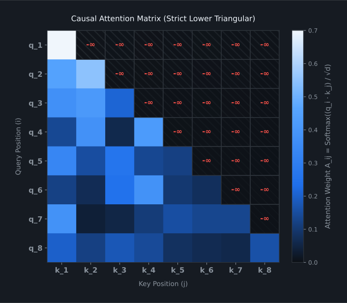
Where $\mathbf{M}$ is the causal autoregressive mask ($M_{ij} = 0$ for $j \le i$, and $M_{ij} = -\infty$ for $j > i$).
Concrete Worked Numerical Example: Causal Attention
Let sequence length $S = 3$ tokens and head dimension $d_k = 2$. Consider the following projected tensors:
$$\mathbf{Q} = \begin{bmatrix} 1.0 & 0.0 \\ 0.0 & 2.0 \\ 1.0 & 1.0 \end{bmatrix}, \quad \mathbf{K} = \begin{bmatrix} 1.0 & 0.0 \\ 1.0 & 1.0 \\ 0.0 & 2.0 \end{bmatrix}, \quad \mathbf{V} = \begin{bmatrix} 10.0 & 1.0 \\ 20.0 & 2.0 \\ 30.0 & 3.0 \end{bmatrix}$$
-
Compute raw dot products $\mathbf{Q}\mathbf{K}^T$: $$\mathbf{Q}\mathbf{K}^T = \begin{bmatrix} (1\cdot 1 + 0\cdot 0) & (1\cdot 1 + 0\cdot 1) & (1\cdot 0 + 0\cdot 2) \\ (0\cdot 1 + 2\cdot 0) & (0\cdot 1 + 2\cdot 1) & (0\cdot 0 + 2\cdot 2) \\ (1\cdot 1 + 1\cdot 0) & (1\cdot 1 + 1\cdot 1) & (1\cdot 0 + 1\cdot 2) \end{bmatrix} = \begin{bmatrix} 1.0 & 1.0 & 0.0 \\ 0.0 & 2.0 & 4.0 \\ 1.0 & 2.0 & 2.0 \end{bmatrix}$$
-
Scale by $\sqrt{d_k} = \sqrt{2} \approx 1.414$: $$\frac{\mathbf{Q}\mathbf{K}^T}{\sqrt{2}} \approx \begin{bmatrix} 0.707 & 0.707 & 0.0 \\ 0.0 & 1.414 & 2.828 \\ 0.707 & 1.414 & 1.414 \end{bmatrix}$$
-
Apply Causal Mask ($-\infty$ in upper triangle): $$\text{Masked Logits} = \begin{bmatrix} 0.707 & -\infty & -\infty \\ 0.0 & 1.414 & -\infty \\ 0.707 & 1.414 & 1.414 \end{bmatrix}$$
-
Apply Row-wise Softmax:
- Row 0: $\text{softmax}([0.707, -\infty, -\infty]) = [1.0, 0.0, 0.0]$ (Token 0 only attends to itself)
- Row 1: $e^0 = 1.0, e^{1.414} \approx 4.112 \implies \mathbf{A}_{1, :} = \left[\frac{1.0}{5.112}, \frac{4.112}{5.112}, 0.0\right] \approx [0.196, 0.804, 0.0]$
- Row 2: $e^{0.707} \approx 2.028, e^{1.414} \approx 4.112, e^{1.414} \approx 4.112 \implies \text{sum} \approx 10.252 \implies \mathbf{A}_{2, :} \approx [0.198, 0.401, 0.401]$
$$\mathbf{A} \approx \begin{bmatrix} 1.000 & 0.000 & 0.000 \\ 0.196 & 0.804 & 0.000 \\ 0.198 & 0.401 & 0.401 \end{bmatrix}$$
-
Aggregate Context Vectors ($\mathbf{O} = \mathbf{A} \mathbf{V}$):
- Row 0: $1.0 \cdot [10.0, 1.0] = [10.0, 1.0]$
- Row 1: $0.196 \cdot [10, 1] + 0.804 \cdot [20, 2] = [1.96 + 16.08, 0.196 + 1.608] = [18.04, 1.804]$
- Row 2: $0.198 \cdot [10, 1] + 0.401 \cdot [20, 2] + 0.401 \cdot [30, 3] = [1.98 + 8.02 + 12.03, 0.198 + 0.802 + 1.203] = [22.03, 2.203]$
$$\mathbf{O} \approx \begin{bmatrix} 10.00 & 1.00 \\ 18.04 & 1.80 \\ 22.03 & 2.20 \end{bmatrix}$$
Notice how Token 2 combines information from all three time-steps, weighted exactly by semantic relevance and causal time boundaries.
4. Multi-Head Attention (MHA)
A single attention calculation forces tokens to focus on a single type of relationship. In natural language, a word has multiple simultaneous relationships (syntactic subject-verb agreement, semantic coreference, emotional sentiment).
Multi-Head Attention splits $D_{model}$ into $H$ independent heads ($d_k = D_{model} / H$):
$$\text{head}_h = \text{Attention}(\mathbf{Q}_h, \mathbf{K}_h, \mathbf{V}_h)$$
$$\text{MHA}(\mathbf{Q}, \mathbf{K}, \mathbf{V}) = \text{Concat}(\text{head}_1, \dots, \text{head}_H) \mathbf{W}_O$$
Each head independently learns to attend to different syntactic and semantic patterns across the sequence.
5. Positional Encoding: Rotary Position Embeddings (RoPE)
Notice an important mathematical detail: Matrix multiplication $\mathbf{Q}\mathbf{K}^T$ treats rows independently. If you shuffle the order of words in a sentence, the attention values remain identical. Attention is permutation invariant.
To give the model a sense of word order, we must inject positional information.
Rotary Position Embedding (RoPE): Step-by-Step Derivation
Su et al. (2021) introduced RoPE, which encodes relative distance by rotating query and key vectors in the 2D complex plane:
For a 2D coordinate $(q_0, q_1)$ at sequence position $m$, define the 2D rotation matrix:
$$\mathbf{R}_{\Theta, m} = \begin{bmatrix} \cos(m\theta) & -\sin(m\theta) \\ \sin(m\theta) & \cos(m\theta) \end{bmatrix}$$
Multiplying $\mathbf{q}_m$ by $\mathbf{R}_{\Theta, m}$ rotates the vector by angle $m\theta$:
$$\tilde{\mathbf{q}}_m = \mathbf{R}_{\Theta, m} \mathbf{q}_m = \begin{bmatrix} q_0 \cos(m\theta) - q_1 \sin(m\theta) \\ q_0 \sin(m\theta) + q_1 \cos(m\theta) \end{bmatrix}$$
Now, consider the dot product between rotated query $\tilde{\mathbf{q}}_m$ at position $m$ and rotated key $\tilde{\mathbf{k}}_n$ at position $n$:
$$\langle \tilde{\mathbf{q}}_m, \tilde{\mathbf{k}}_n \rangle = (\mathbf{R}_{\Theta, m} \mathbf{q}_m)^T (\mathbf{R}_{\Theta, n} \mathbf{k}_n) = \mathbf{q}_m^T \left( \mathbf{R}_{\Theta, m}^T \mathbf{R}_{\Theta, n} \right) \mathbf{k}_n$$
Since 2D rotation matrices are orthogonal ($\mathbf{R}_{\Theta, m}^T = \mathbf{R}_{\Theta, -m}$) and commute:
$$\mathbf{R}_{\Theta, m}^T \mathbf{R}_{\Theta, n} = \mathbf{R}_{\Theta, -m} \mathbf{R}_{\Theta, n} = \mathbf{R}_{\Theta, n - m} = \begin{bmatrix} \cos((n - m)\theta) & -\sin((n - m)\theta) \\ \sin((n - m)\theta) & \cos((n - m)\theta) \end{bmatrix}$$
Therefore:
$$\langle \tilde{\mathbf{q}}_m, \tilde{\mathbf{k}}_n \rangle = \mathbf{q}_m^T \mathbf{R}_{\Theta, n - m} \mathbf{k}_n$$
The dot product depends strictly on the relative distance $(n - m)$ between tokens! Tokens separated by 3 positions have the identical rotational offset whether they appear at positions $(0, 3)$ or $(4000, 4003)$. RoPE enables models to generalize naturally to sequence lengths unseen during training.
6. Prototypical NetCL Implementation
NetCL provides end-to-end tokenization and Rotary Multi-Head Attention:
import numpy as np
from netcl.text import BPETokenizer, ChatFormat
from netcl.core.device import manager
from netcl.core.tensor import Tensor
import netcl.autograd as ag

# 1. Byte-level BPE Tokenization
tok = BPETokenizer()
tok.train_from_iterator(["Hello world!", "Attention is all you need."])
tokens = tok.encode("Hello world!")
print("Token IDs:", tokens)
print("Reconstructed text:", tok.decode(tokens))

# 2. Multi-Head Attention on OpenCL Device
q = manager.default("auto").queue
from netcl.nn.transformer import RotaryAttention

attn = RotaryAttention(
    queue=q,
    dim=256,
    n_heads=4,
    n_kv_heads=4,
    max_seq_len=512,
)

# Batch of 2 sequences, length 16, dimension 256
x_batch = Tensor.from_host(q, np.random.randn(2, 16, 256).astype(np.float32))

with ag.Tape() as tape:
    x_node = ag.tensor(x_batch)
    out = attn(x_node)

print(f"Attention output shape: {out.value.shape}")
assert out.value.shape == (2, 16, 256)
Related Documentation
- Text API Reference: Tokenizer training, regex splitting, and chat templating.
- Concepts: Transformer: Decoder blocks, SwiGLU feed-forward networks, and KV-cache.
Next Steps in the Curriculum
Notice that computing $\mathbf{Q}\mathbf{K}^T$ materializes an $(S \times S)$ matrix in memory. For long sequences ($S = 8,192$), storing this matrix consumes gigabytes of VRAM.
Proceed to Chapter 8: Hardware Realities & FlashAttention to learn how memory bandwidth governs GPU speed and how tiled online Softmax solves the attention memory bottleneck.