
Neural Building Blocks: From Linear Projections to Deep Representations
Neural Building Blocks: From Linear Projections to Deep Representations
In Chapter 3: Optimization Algorithms, we mastered the algorithms that step parameters down a loss hill.
Now we turn to the structure of the model itself: How do we construct a mathematical function that can recognize handwritten digits, detect objects in images, or generate human language?
This chapter reveals why linear transformations alone are incapable of learning complex patterns, how non-linear activation functions bend high-dimensional space, and why weight initialization is critical to prevent vanishing or exploding gradients.
1. Core Intuition: Folding a Flat Sheet of Paper
Imagine you have a flat sheet of paper with red dots in the center and blue dots surrounding them in a circle.
       Blue (o)      Blue (o)
              Red (*)
       Blue (o)      Blue (o)
Can you separate the red dots from the blue dots with a single straight cut of scissors? - No. A straight cut (a linear boundary) can only divide space into two flat half-planes. No single line can isolate the center from the perimeter. - Now, pick up the sheet of paper and fold it or crumple it into a 3D shape. - In this folded space, the red dots pop up into a crease. Now, a single flat slice of a knife cleanly cuts off the red crease while leaving the blue dots behind!
Linear transformations stretch, rotate, and scale the paper. Non-linear activation functions fold the paper. Stacking both creates a deep neural network capable of carving out arbitrary decision boundaries.
2. Linear Projections: The Matrix Transformation
The fundamental workhorse of deep learning is the affine linear layer:
$$\mathbf{y} = \mathbf{x}\mathbf{W} + \mathbf{b}$$
Where: - $\mathbf{x} \in \mathbb{R}^{1 \times D_{in}}$ is the input feature vector. - $\mathbf{W} \in \mathbb{R}^{D_{in} \times D_{out}}$ is the learnable weight matrix. - $\mathbf{b} \in \mathbb{R}^{1 \times D_{out}}$ is the learnable bias offset.
The Collapse Theorem: Why Deep Linear Networks are Pointless
What happens if you stack two linear layers without an activation function in between?
$$\mathbf{h} = \mathbf{x}\mathbf{W}_1 + \mathbf{b}_1$$
$$\mathbf{y} = \mathbf{h}\mathbf{W}_2 + \mathbf{b}_2 = (\mathbf{x}\mathbf{W}_1 + \mathbf{b}_1)\mathbf{W}_2 + \mathbf{b}_2 = \mathbf{x}(\mathbf{W}_1\mathbf{W}_2) + (\mathbf{b}_1\mathbf{W}_2 + \mathbf{b}_2)$$
Notice that $\mathbf{W}_{eff} = \mathbf{W}_1\mathbf{W}_2$ is just another matrix, and $\mathbf{b}_{eff} = \mathbf{b}_1\mathbf{W}_2 + \mathbf{b}_2$ is just another bias vector.
Theorem: A stack of 100 consecutive linear layers is mathematically equivalent to a single linear layer. Without non-linearities, depth provides zero representational power.
3. Non-Linear Activation Functions
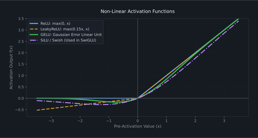
To prevent depth collapse, every linear projection must be followed by an elementwise non-linear function $\sigma(z)$.
1. Sigmoid and Tanh (The Early Era)
$$\sigma_{sigmoid}(z) = \frac{1}{1 + e^{-z}}, \quad \sigma_{tanh}(z) = \frac{e^z - e^{-z}}{e^z + e^{-z}}$$
The Vanishing Gradient Problem: When input $z$ is large ($|z| > 4$), the output of Sigmoid saturates at 0 or 1. Its derivative is:
$$\sigma'(z) = \sigma(z)(1 - \sigma(z)) \approx 0$$
Multiplying numbers near zero through the chain rule causes gradients to vanish exponentially as they propagate backward to earlier layers, halting learning in deep networks.
2. Rectified Linear Unit (ReLU)
Nair & Hinton (2010) introduced ReLU, which revolutionized deep learning:
$$\text{ReLU}(z) = \max(0, z)$$
$$\frac{d}{dz}\text{ReLU}(z) = \begin{cases} 1 & \text{if } z > 0 \\ 0 & \text{if } z \le 0 \end{cases}$$
Why ReLU transformed the field:
- Non-saturating gradient: For all positive activations, the gradient is exactly $1.0$. Gradients flow backward across dozens of layers without decay.
- Extreme computational speed: Evaluating $\max(0, z)$ on GPU hardware takes a single instruction cycle, avoiding expensive transcendental operations like exp().
The Dying ReLU Pathology: If a neuron's weights receive an unlucky update that pushes its output negative for all samples in the dataset, its gradient is permanently 0. The neuron becomes dead and never recovers.
3. Modern Activations: GELU & SwiGLU
In modern Large Language Models and Vision Transformers, smooth activations replace hard-clipping ReLUs:
- GELU (Gaussian Error Linear Unit): Weights inputs by the cumulative distribution function of the normal distribution:
$$\text{GELU}(z) = z \cdot \Phi(z) = z \cdot \frac{1}{2} \left[ 1 + \text{erf}\left(\frac{z}{\sqrt{2}}\right) \right]$$
- SwiGLU (Swish Gated Linear Unit): Used in LLaMA-style transformer decoders:
$$\text{SwiGLU}(x) = (\text{Swish}(x W_{gate})) \odot (x W_{up})$$
4. The Weight Initialization Problem
How should weights $\mathbf{W}$ be initialized before training starts?
Why Zero Initialization Fails
If all weights are initialized to zero ($\mathbf{W} = \mathbf{0}$): 1. Every hidden neuron computes identical values: $z_j = 0 \cdot x + 0 = 0$. 2. Backpropagation computes identical gradients for every neuron: $\frac{\partial \mathcal{L}}{\partial w_{ij}} = \frac{\partial \mathcal{L}}{\partial w_{ik}}$. 3. All neurons update identically and learn the exact same feature. The network suffers from symmetry lock and behaves as if it only had a single neuron.
Variance Preservation (Xavier & Kaiming Initialization)
To break symmetry, we must initialize weights with small random noise. However: - If weights are too large ($Var(W) \gg 1$), activations explode exponentially with depth ($10^{30} \to \text{NaN}$). - If weights are too small ($Var(W) \ll 1$), activations shrink exponentially toward zero ($10^{-30} \to 0$).
We need the variance of activations to remain constant across all layers: $\text{Var}(y) = \text{Var}(x)$.
For a layer with $D_{in}$ inputs and $D_{out}$ outputs: - Xavier (Glorot) Initialization (for Tanh / Sigmoid):
$$\mathbf{W} \sim \mathcal{N}\left(0, \frac{2}{D_{in} + D_{out}}\right)$$
- Kaiming (He) Initialization (for ReLU / GELU): Because ReLU zeroes out half of all activations, the output variance is cut in half. To compensate, we double the initial variance:
$$\mathbf{W} \sim \mathcal{N}\left(0, \frac{2}{D_{in}}\right)$$
5. Prototypical NetCL Implementation
NetCL provides modular, object-oriented layers in netcl.nn that automatically handle Kaiming initialization and forward execution:
import numpy as np
import netcl.autograd as ag
import netcl.nn as nn
from netcl.core.device import manager
from netcl.core.tensor import Tensor

q = manager.default("auto").queue

# 1. Construct an expressive Multi-Layer Perceptron (MLP)
class MultiLayerPerceptron(nn.Module):
    def __init__(self, queue, in_features, hidden_dim, out_features):
        super().__init__()
        # Layers automatically apply Kaiming He initialization
        self.fc1 = nn.Linear(queue, in_features, hidden_dim)
        self.act1 = nn.ReLU()
        self.fc2 = nn.Linear(queue, hidden_dim, hidden_dim)
        self.act2 = nn.GELU()
        self.fc3 = nn.Linear(queue, hidden_dim, out_features)

    def forward(self, x):
        h = self.act1(self.fc1(x))
        h = self.act2(self.fc2(h))
        return self.fc3(h)

# 2. Or compose sequentially with nn.Sequential
model = nn.Sequential(
    nn.Linear(q, 784, 256),
    nn.ReLU(),
    nn.Dropout(p=0.1),
    nn.Linear(q, 256, 128),
    nn.GELU(),
    nn.Linear(q, 128, 10),
)

# 3. Verify forward pass on GPU
batch_input = Tensor.from_host(q, np.random.randn(16, 784).astype(np.float32))

with ag.Tape() as tape:
    x_node = ag.tensor(batch_input)
    logits = model(x_node)

print(f"Logits shape: {logits.value.shape}")
assert logits.value.shape == (16, 10)
Related Documentation
- NN API Reference: Full method signatures for
Linear,Conv2d,BatchNorm2d,Sequential, and initialization utilities. - Concepts: Linear Layers: Details on OpenCL GEMM matrix multiplication kernels.
- Concepts: ReLU: GPU kernel implementation of non-linear activations.
Now that you know how to build dense multi-layer networks, how do we systematically train their parameters without getting stuck in saddle points or oscillating uncontrollably?
Proceed to Chapter 4: Optimization Algorithms to master Mini-Batch SGD, Momentum, and decoupled AdamW.