knowledge

Optimization Algorithms: The Science of Stepping Downhill

In Chapter 2: Calculus, Gradients & Computational Graphs, we discovered how reverse-mode automatic differentiation computes the exact gradient vector $\nabla_\theta \mathcal{L}$.

Knowing which way is downhill is only half the battle. How far should you step? What if the ground under your feet is a narrow canyon with steep cliffs on both sides?

This chapter covers the mathematical evolution of modern deep learning optimizers: from Vanilla Gradient Descent to Momentum, RMSprop, Adam, and the AdamW weight decay breakthrough.

1. Core Intuition: The Rolling Heavy Marble

Imagine dropping a tiny plastic bead into a bumpy bowl. - If you push it directly downhill, it will zig-zag wildly between the steep walls of the bowl. - Now replace the bead with a heavy iron bowling ball. - As the bowling ball rolls, its inertia builds momentum in the direction of continuous progress (along the valley floor) while cancelling out the chaotic side-to-side bounces.

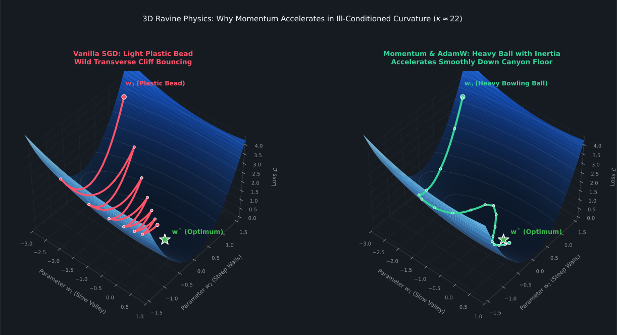
Optimization Trajectories in Ravine: Vanilla SGD vs Momentum & AdamW

Modern optimization is the science of designing mathematical inertia and adaptive friction to guide parameters down high-dimensional landscapes safely and quickly.

2. Stochastic Gradient Descent (SGD)

Full Batch vs. Mini-Batch

In an ideal mathematical world, we would compute the gradient over all $M$ samples in the dataset:

$$\mathbf{g} = \frac{1}{M} \sum_{i=1}^M \nabla_\theta \ell_i(\theta)$$

In real applications, datasets contain millions of images or tokens that cannot fit into GPU memory simultaneously. Stochastic Gradient Descent (SGD) approximates the true gradient by computing it over a small, randomized mini-batch $\mathcal{B}$ of size $B$ (typically 32 to 512 samples):

$$\mathbf{g}_t = \frac{1}{B} \sum_{i \in \mathcal{B}_t} \nabla_\theta \ell_i(\theta_t)$$

The parameter update rule is:

$$\theta_{t+1} = \theta_t - \eta \cdot \mathbf{g}_t$$

Where $\eta > 0$ is the learning rate.

The Failure Mode of Vanilla SGD: Ill-Conditioned Curvature

In deep networks, the loss surface is rarely isotropic (like a round bowl). Instead, it forms ill-conditioned ravines: surfaces where the curvature is steep in one direction but flat along the path toward the minimum.

Because $\nabla \mathcal{L}$ is dominated by the steep direction, vanilla SGD bounces violently back and forth across the canyon walls, making agonizingly slow progress along the valley floor.

3. Momentum: Harnessing Physical Inertia

To damp oscillations across steep directions and accelerate along flat ravines, Polyak (1964) introduced Momentum.

Instead of stepping directly proportional to the current gradient $\mathbf{g}_t$, we maintain an exponential moving average of past gradients, representing physical velocity $\mathbf{v}_t$:

$$\mathbf{v}_t = \beta \mathbf{v}_{t-1} + (1 - \beta) \mathbf{g}_t$$

$$\theta_{t+1} = \theta_t - \eta \cdot \mathbf{v}_t$$

Where $\beta \in [0, 1)$ is the momentum coefficient (standard default: $\beta = 0.9$).

Why this works: - Along oscillating directions, gradients alternate signs ($+,-,+,-$). The moving average sums them to near zero, dampening jitter. - Along consistent directions, gradients point in the same direction ($+,+,+,+$). The velocity accelerates, compounding speed by a factor of $\frac{1}{1 - \beta} = \frac{1}{1 - 0.9} = 10\times$.

4. RMSprop: Adaptive Per-Parameter Learning Rates

Different parameters in a network have vastly different scales. Features in an embedding layer may receive infrequent updates, while weights in the first layer may receive massive gradient surges.

Tieleman & Hinton (2012) introduced RMSprop (Root Mean Square Propagation). Instead of applying the same global learning rate $\eta$ to all parameters, RMSprop normalizes each coordinate by the square root of its recent gradient variance:

$$\mathbf{s}_t = \alpha \mathbf{s}_{t-1} + (1 - \alpha) \mathbf{g}_t^2$$

$$\theta_{t+1} = \theta_t - \frac{\eta}{\sqrt{\mathbf{s}_t} + \epsilon} \odot \mathbf{g}_t$$

Where $\alpha \approx 0.99$ and $\epsilon \approx 10^{-8}$ prevents division by zero. - If a parameter has historically large gradients, $\sqrt{\mathbf{s}_t}$ is large, which automatically shrinks its effective step size. - If a parameter has historically small gradients, $\sqrt{\mathbf{s}_t}$ is small, which automatically amplifies its step size.

5. Adam: Combining Momentum and Adaptive Scale

Kingma & Ba (2014) synthesized the benefits of Momentum (first moment $\mathbf{m}_t$) and RMSprop (second moment $\mathbf{v}_t$) into Adam (Adaptive Moment Estimation).

Step 1: Exponential Moving Averages

$$\mathbf{m}_t = \beta_1 \mathbf{m}_{t-1} + (1 - \beta_1) \mathbf{g}_t \quad (\text{Mean / Velocity})$$

$$\mathbf{v}_t = \beta_2 \mathbf{v}_{t-1} + (1 - \beta_2) \mathbf{g}_t^2 \quad (\text{Variance / Energy})$$

Standard defaults: $\beta_1 = 0.9, \beta_2 = 0.999$.

Step 2: Bias Correction

Because $\mathbf{m}_0 = \mathbf{0}$ and $\mathbf{v}_0 = \mathbf{0}$, both vectors are biased toward zero during the initial training steps. We correct this by scaling by the sum of geometric weights:

$$\hat{\mathbf{m}}_t = \frac{\mathbf{m}_t}{1 - \beta_1^t}, \quad \hat{\mathbf{v}}_t = \frac{\mathbf{v}_t}{1 - \beta_2^t}$$

As $t \to \infty$, $\beta^t \to 0$ and the correction factor approaches 1.0.

Step 3: Parameter Update

$$\theta_{t+1} = \theta_t - \eta \cdot \frac{\hat{\mathbf{m}}_t}{\sqrt{\hat{\mathbf{v}}_t} + \epsilon}$$

6. The AdamW Breakthrough: Decoupled Weight Decay

For years, researchers struggled with the fact that L2 regularization in Adam failed to generalize as well as SGD with momentum. Loshchilov & Hutter (2019) identified the mathematical root cause.

In classic optimization, L2 regularization minimizes the objective $\mathcal{L}(\theta) + \frac{1}{2} \lambda \|\theta\|^2$. Taking the derivative yields:

$$\nabla \mathcal{L}_{reg} = \mathbf{g}_t + \lambda \theta_t$$

When this penalized gradient is plugged into Adam, the update becomes:

$$\Delta \theta_t \approx - \frac{\eta}{\sqrt{\hat{\mathbf{v}}_t}} (\dots + \lambda \theta_t)$$

The Pathology: The weight decay term $\lambda \theta_t$ is divided by $\sqrt{\hat{\mathbf{v}}_t}$! - Parameters with frequent, large gradients experience virtually no weight decay. - Parameters with small, sparse gradients experience massive, disproportionate shrinkage.

The Solution (AdamW): Decouple weight decay entirely from the adaptive gradient moment calculation:

$$\theta_{t+1} = \theta_t - \eta \left( \frac{\hat{\mathbf{m}}_t}{\sqrt{\hat{\mathbf{v}}_t} + \epsilon} + \lambda \theta_t \right)$$

Weights decay strictly proportional to their magnitude and the learning rate, restoring proper regularization. AdamW is now the standard optimizer across all modern LLMs and vision backbones.

7. Learning Rate Schedules: Warmup & Cosine Annealing

A constant learning rate $\eta$ is suboptimal. Modern training pipelines employ two essential phases:

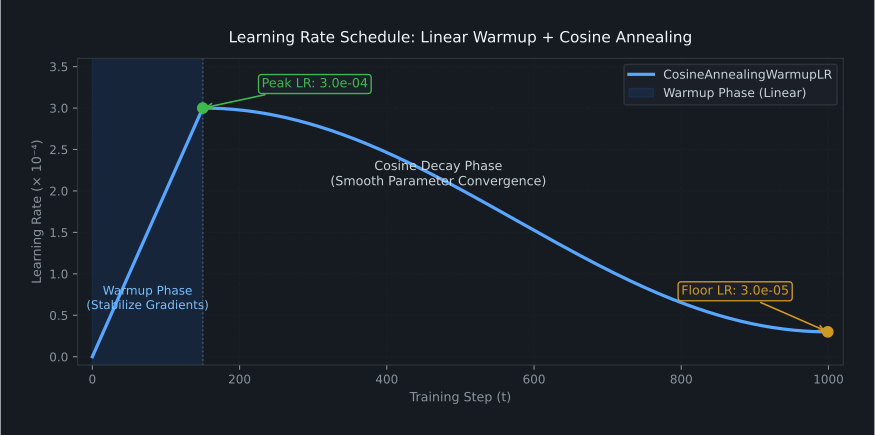
Learning Rate Schedule: Warmup and Cosine Annealing

Linear Warmup: For the first few hundred steps, the learning rate scales linearly from near zero up to $\eta_{max}$. This prevents large, erratic gradients from destabilizing uninitialized weights.
Cosine Annealing Decay: The learning rate decays smoothly according to a cosine curve down to $\eta_{min}$, allowing fine-grained convergence into narrow loss minima.

8. NetCL Implementation & Fused Kernels

In netcl, all optimizers execute as single-pass fused OpenCL kernels. The moments $m_t, v_t$ and parameters $\theta_t$ are updated directly within GPU registers without allocating intermediate arrays:

import netcl.optim as opt
from netcl.nn import Linear, Sequential
from netcl.core.device import manager

q = manager.default("auto").queue

# 1. Instantiate neural network
model = Sequential(Linear(q, 784, 128), Linear(q, 128, 10))

# 2. Configure AdamW with decoupled weight decay
optimizer = opt.AdamW(
    model.parameters(),
    lr=1e-3,
    betas=(0.9, 0.999),
    weight_decay=1e-2,
)

# 3. Configure Warmup Cosine scheduler
scheduler = opt.WarmupCosine(
    optimizer,
    warmup_steps=100,
    total_steps=1000,
    min_lr=1e-5,
)

# In the training loop:
# tape.backward(loss)
optimizer.step(max_norm=1.0)  # Fused gradient clipping + AdamW update
optimizer.zero_grad()
scheduler.step()

Concepts: AdamW: Deep dive into the OpenCL C kernel code for fused updates.
Optimizer API Reference: Signatures for SGD, Adam, AdamW, RMSprop, and schedulers.
Tutorial: MNIST Digit Classifier: See AdamW in action on a real dataset.

Next Steps in the Curriculum

Now that you master optimization and autograd, how do we process structured spatial data like 2D images without blowing up parameter counts?

Proceed to Chapter 5: Convolutions & Spatial Vision to explore 2D sliding filters, the im2col GEMM formulation, and Winograd minimal filtering.

← Module 3: Neural Building Blocks 🧭 Curriculum Hub Next: Convolutions & Vision →