
What is Machine Learning? Foundations from First Principles
What is Machine Learning? Foundations from First Principles
Machine learning is often described with intimidating jargon: non-convex loss manifolds, statistical regularization, and high-dimensional parameter spaces.
At its mechanical core, machine learning is automated curve fitting on steroids.
This chapter starts from absolute zero. It introduces the mental model of parameters, feature spaces, targets, and loss landscapes, and demonstrates how these mathematical abstractions map directly to physical OpenCL memory buffers in netcl.
1. Core Intuition: A Guessing Machine with a Dial
Imagine you have a black box with an input slot, an output screen, and a rotary knob on top.
Parameter Dial: w"] Box --> YHat["Prediction (y_hat)"] YHat --> Loss["Error / Loss L(w)
Compare with Truth y"] Truth["Ground Truth (y)"] --> Loss
- You feed an input number $x = 2$ into the box.
- The box computes a prediction $\hat{y} = w \cdot x$. If the knob is set to $w = 1$, the box outputs $\hat{y} = 2$.
- You check the correct answer (ground truth): $y = 6$.
- The error (or loss) is the discrepancy between what the box predicted and reality: $e = \hat{y} - y = 2 - 6 = -4$.
- To fix the error, you turn the knob $w$ clockwise to increase the output. If you turn it to $w = 3$, the box outputs $\hat{y} = 3 \cdot 2 = 6$. The error is zero.
Machine learning is nothing more than scaling this mechanism from 1 knob to millions (or billions) of knobs simultaneously.
2. Mathematical Formalization
Let us translate this intuition into formal vector mathematics.
Features (Inputs)
A single data point is represented as a feature vector $\mathbf{x} \in \mathbb{R}^D$, where $D$ is the number of measurable attributes (e.g. pixels in an image or historical house prices). In matrix form, a mini-batch of $N$ independent samples is grouped into a feature matrix:
$$\mathbf{X} \in \mathbb{R}^{N \times D}$$
Parameters (Weights and Biases)
The knobs inside the model are parameters: - Weight Matrix $\mathbf{W} \in \mathbb{R}^{D \times M}$: Multiplicative scaling factors that determine how strongly each input feature influences each output. - Bias Vector $\mathbf{b} \in \mathbb{R}^M$: Additive offsets that allow the model to output non-zero values even when the input is zero.
Formal Vector Transformation
Together, the weights and biases define an affine geometric transformation:
$$\hat{\mathbf{Y}} = \mathbf{X}\mathbf{W} + \mathbf{b}$$
Zero Hidden Premises: Symbol Breakdown
| Symbol | Mathematical Domain | OpenCL Hardware & Memory Mapping |
|---|---|---|
| $\mathbf{X}$ | $\mathbb{R}^{N \times D}$ | Mini-batch input matrix buffer ($N \times D \times 4$ bytes in VRAM) |
| $N$ | $\mathbb{N}^+$ | Batch size (number of independent examples processed in parallel) |
| $D$ | $\mathbb{N}^+$ | Input dimension (number of features per sample) |
| $\mathbf{W}$ | $\mathbb{R}^{D \times M}$ | Weight matrix buffer ($D \times M \times 4$ bytes in VRAM) |
| $M$ | $\mathbb{N}^+$ | Output dimension (number of target predictions or logits) |
| $\mathbf{b}$ | $\mathbb{R}^M$ | Additive bias vector broadcast across rows ($M \times 4$ bytes) |
| $\hat{\mathbf{Y}}$ | $\mathbb{R}^{N \times M}$ | Model prediction matrix buffer ($N \times M \times 4$ bytes in VRAM) |
| $\mathbf{Y}$ | $\mathbb{R}^{N \times M}$ | Ground-truth target matrix buffer ($N \times M \times 4$ bytes in VRAM) |
Concrete Worked Numerical Example: Affine Projection
Let $N = 2$ samples, $D = 2$ input features, and $M = 1$ output prediction:
$$\mathbf{X} = \begin{bmatrix} 1.0 & 2.0 \\ 3.0 & 0.5 \end{bmatrix}, \quad \mathbf{W} = \begin{bmatrix} 0.4 \\ -0.5 \end{bmatrix}, \quad \mathbf{b} = \begin{bmatrix} 0.1 \end{bmatrix}$$
Step 1: Compute matrix product $\mathbf{X}\mathbf{W}$: - Sample 1: $1.0 \cdot (0.4) + 2.0 \cdot (-0.5) = 0.4 - 1.0 = -0.6$ - Sample 2: $3.0 \cdot (0.4) + 0.5 \cdot (-0.5) = 1.2 - 0.25 = 0.95$
$$\mathbf{X}\mathbf{W} = \begin{bmatrix} -0.6 \\ 0.95 \end{bmatrix}$$
Step 2: Add broadcast bias vector $\mathbf{b}$:
$$\hat{\mathbf{Y}} = \begin{bmatrix} -0.6 + 0.1 \\ 0.95 + 0.1 \end{bmatrix} = \begin{bmatrix} -0.5 \\ 1.05 \end{bmatrix}$$
3. The Loss Landscape: Measuring Mistake Severity
To systematically adjust the knobs, we need a mathematical function that quantifies the severity of errors across the entire dataset. This is the Loss Function $\mathcal{L}(\mathbf{W}, \mathbf{b})$.
Mean Squared Error (MSE): Formal Definition & Derivation
For regression problems, the standard objective is the squared Euclidean distance between predictions and targets:
$$\mathcal{L}_{MSE}(\mathbf{W}, \mathbf{b}) = \frac{1}{N} \sum_{i=1}^N \|\hat{\mathbf{y}}_i - \mathbf{y}_i\|^2 = \frac{1}{N} \sum_{i=1}^N \sum_{j=1}^M (\hat{y}_{ij} - y_{ij})^2$$
In compact matrix trace notation:
$$\mathcal{L}_{MSE}(\mathbf{W}, \mathbf{b}) = \frac{1}{N} \|\mathbf{X}\mathbf{W} + \mathbf{b} - \mathbf{Y}\|_F^2$$
Step-by-Step Gradient Derivation
To update $\mathbf{W}$ via gradient descent, we differentiate the scalar loss $\mathcal{L}$ with respect to the matrix $\mathbf{W}$.
Let error matrix $\mathbf{E} = \hat{\mathbf{Y}} - \mathbf{Y} = \mathbf{X}\mathbf{W} + \mathbf{b} - \mathbf{Y} \in \mathbb{R}^{N \times M}$. The scalar loss is $\mathcal{L} = \frac{1}{N} \sum_{i, j} E_{ij}^2$.
By the chain rule:
$$\frac{\partial \mathcal{L}}{\partial W_{kj}} = \sum_{i=1}^N \frac{\partial \mathcal{L}}{\partial E_{ij}} \frac{\partial E_{ij}}{\partial W_{kj}}$$
- Since $\mathcal{L} = \frac{1}{N} \sum E_{ij}^2$, the partial derivative is: $$\frac{\partial \mathcal{L}}{\partial E_{ij}} = \frac{2}{N} E_{ij}$$
- Since $E_{ij} = \sum_{r=1}^D X_{ir} W_{rj} + b_j - Y_{ij}$, differentiating with respect to $W_{kj}$ selects $r = k$: $$\frac{\partial E_{ij}}{\partial W_{kj}} = X_{ik}$$
- Substituting these back into the summation: $$\frac{\partial \mathcal{L}}{\partial W_{kj}} = \frac{2}{N} \sum_{i=1}^N X_{ik} E_{ij} = \frac{2}{N} \sum_{i=1}^N (\mathbf{X}^T)_{ki} E_{ij}$$
In matrix form, the entire gradient is a single matrix multiplication:
$$\nabla_{\mathbf{W}} \mathcal{L} = \frac{2}{N} \mathbf{X}^T (\hat{\mathbf{Y}} - \mathbf{Y})$$
Similarly, for the bias vector:
$$\nabla_{\mathbf{b}} \mathcal{L} = \frac{2}{N} \sum_{i=1}^N (\hat{\mathbf{y}}_i - \mathbf{y}_i) = \frac{2}{N} \mathbf{1}^T (\hat{\mathbf{Y}} - \mathbf{Y})$$
Concrete Worked Numerical Step: Error & Loss
Using our sample predictions $\hat{\mathbf{Y}} = [-0.5, 1.05]^T$ and ground-truth targets $\mathbf{Y} = [1.0, 2.0]^T$:
- Compute prediction residuals: $$\mathbf{E} = \hat{\mathbf{Y}} - \mathbf{Y} = \begin{bmatrix} -0.5 - 1.0 \\ 1.05 - 2.0 \end{bmatrix} = \begin{bmatrix} -1.5 \\ -0.95 \end{bmatrix}$$
- Square each residual: $$(-1.5)^2 = 2.25, \quad (-0.95)^2 = 0.9025$$
- Average across $N=2$ samples: $$\mathcal{L}_{MSE} = \frac{2.25 + 0.9025}{2} = \frac{3.1525}{2} = 1.57625$$
- Compute the analytical gradient $\nabla_{\mathbf{W}} \mathcal{L}$: $$\nabla_{\mathbf{W}} \mathcal{L} = \frac{2}{2} \begin{bmatrix} 1.0 & 3.0 \\ 2.0 & 0.5 \end{bmatrix} \begin{bmatrix} -1.5 \\ -0.95 \end{bmatrix} = \begin{bmatrix} 1.0(-1.5) + 3.0(-0.95) \\ 2.0(-1.5) + 0.5(-0.95) \end{bmatrix} = \begin{bmatrix} -1.5 - 2.85 \\ -3.0 - 0.475 \end{bmatrix} = \begin{bmatrix} -4.35 \\ -3.475 \end{bmatrix}$$
Because the gradient is negative, the update $\mathbf{W} \leftarrow \mathbf{W} - \alpha \nabla_{\mathbf{W}} \mathcal{L}$ will increase both weights, reducing our under-prediction error!
The Loss Landscape
Imagine the loss $\mathcal{L}$ as the altitude of a mountainous terrain, where the coordinates on the ground represent the values of parameters $w_1$ and $w_2$.
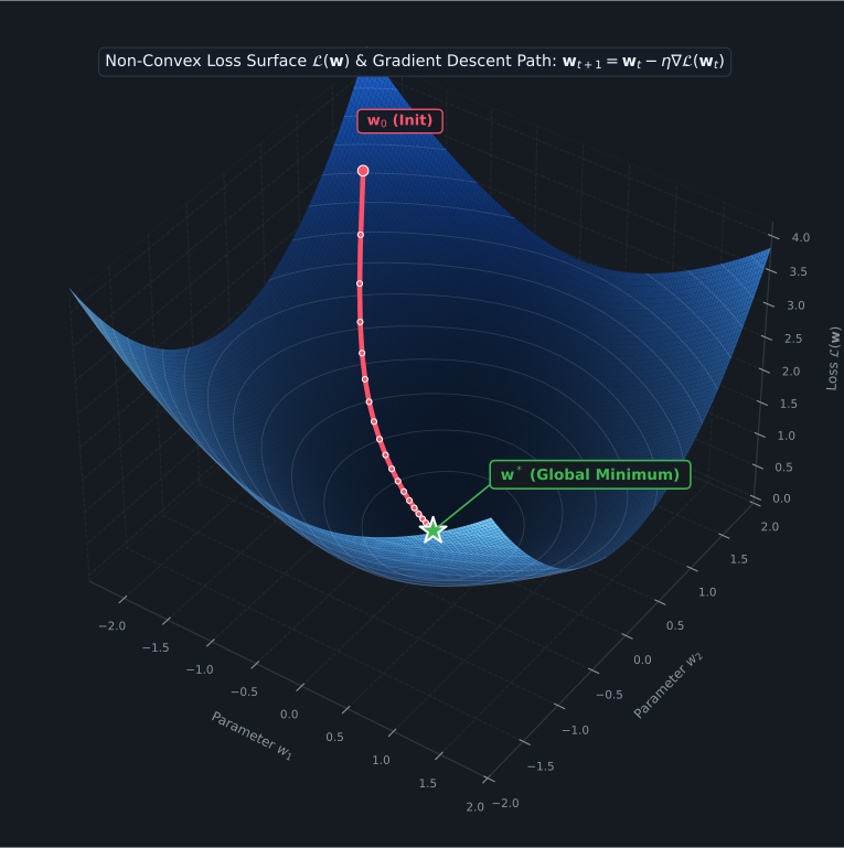
The fundamental goal of machine learning is to navigate from the high-altitude peaks down into the lowest valley, finding optimal parameters $\theta^* = \{\mathbf{W}^*, \mathbf{b}^*\}$ that minimize $\mathcal{L}$.
4. Hardware Reality: From Math to GPU Memory
On a GPU, mathematical vectors cannot exist as abstract concepts. They are physical arrays of 32-bit floating point numbers stored in High Bandwidth Memory (VRAM).
In netcl:
- A matrix $\mathbf{X} \in \mathbb{R}^{32 \times 784}$ is represented as a contiguous buffer of $32 \times 784 \times 4 \text{ bytes} \approx 100 \text{ KB}$ of device memory (cl_mem).
- Matrix multiplication $\mathbf{X}\mathbf{W}$ executes as hundreds of concurrent GPU threads, where each thread computes a dot product in parallel.
- The command queue is the physical pipeline through which the CPU orders the GPU cores to execute these calculations.
5. From Theory to NetCL Implementation
Here is how the theoretical formulation above maps directly into executable NetCL code:
import numpy as np
from netcl.core.device import manager
from netcl.core.tensor import Tensor
import netcl.autograd as ag

# 1. Connect to GPU hardware queue
dev = manager.default("auto")
q = dev.queue

# 2. Features X: 100 samples, 4 features each
X_np = np.random.randn(100, 4).astype(np.float32)
# Targets y: true relationship is y = 2*x0 - 3*x1 + x2 + 0.5
y_np = (2.0 * X_np[:, 0:1] - 3.0 * X_np[:, 1:2] + X_np[:, 2:3] + 0.5).astype(np.float32)

X = Tensor.from_host(q, X_np)
y = Tensor.from_host(q, y_np)

# 3. Parameters W (4x1) and bias b (1,) initialized randomly
W = Tensor.from_host(q, np.random.randn(4, 1).astype(np.float32) * 0.1)
b = Tensor.from_host(q, np.zeros((1,), dtype=np.float32))

# 4. Predict and evaluate Loss inside Autograd Tape
with ag.Tape() as tape:
    # Wrap raw GPU buffers into autograd nodes
    X_node = ag.tensor(X)
    y_node = ag.tensor(y)
    W_node = ag.tensor(W)
    b_node = ag.tensor(b)

    # Affine transformation: y_hat = X @ W + b
    y_hat = ag.add(ag.matmul(X_node, W_node), b_node)

    # Mean Squared Error: L = mean((y_hat - y)^2)
    diff = y_hat - y_node
    loss = ag.mean(diff * diff)

print(f"Initial Mean Squared Error: {loss.value.to_host()[0]:.4f}")
Next Steps in the Curriculum
Now that you understand what a model and a loss landscape are, how do we systematically turn the knobs to reach the bottom of the valley?
Proceed to Chapter 2: Calculus, Gradients & Computational Graphs to learn how derivatives guide parameters down the loss hill.