
Normalization & Regularization: Stabilizing Deep Networks
Normalization & Regularization: Stabilizing Deep Networks
In Chapter 5: Convolutions & Computer Vision, we saw how deep residual networks enable architectures with dozens of layers.
However, as a deep network trains, an insidious problem emerges: each layer modifies its weights at every step. This means the distribution of inputs to subsequent layers is constantly drifting. A layer that learned to process inputs centered around zero suddenly receives activations centered around 100 with massive variance.
This chapter covers the mathematical foundations of normalization (Batch Normalization, Layer Normalization, and RMSNorm) and regularization (Dropout and Weight Decay) to stabilize training dynamics.
1. Core Intuition: The Audio Soundboard
Imagine a music studio with 50 amplifiers connected in series: - If each amplifier increases the volume by just $10\%$, the audio will scream into deafening, distorted feedback by amplifier 10 ($1.1^{10} \approx 2.6$, $1.1^{50} \approx 117$). - If each amplifier decreases the volume by $10\%$, the sound vanishes into inaudible silence ($0.9^{50} \approx 0.005$).
To get crystal-clear audio through 50 stages, an audio engineer inserts an automatic leveler (limiter) between every amplifier. The leveler measures the current volume, resets it to a standard comfortable volume, and passes it forward.
Normalization layers are automatic volume limiters for neural network activations.
2. Batch Normalization (BatchNorm)
Ioffe & Szegedy (2015) introduced Batch Normalization to stabilize training in deep convolutional networks.
Step 1: Compute Mini-Batch Statistics
Given a mini-batch $\mathcal{B} = \{x_1, \dots, x_N\}$ for a specific channel feature:
Zero Hidden Premises: Symbol Breakdown
| Symbol | Mathematical Domain | Physical Role & Hardware Meaning |
|---|---|---|
| $N$ | $\mathbb{N}^+$ | Mini-batch dimension (number of independent sequences/images) |
| $D$ | $\mathbb{N}^+$ | Feature / channel dimension (e.g. 4,096 hidden units) |
| $\mathbf{X} \in \mathbb{R}^{N \times D}$ | Input activation buffer in GPU VRAM ($N \times D \times 4$ bytes) | |
| $\mu_{\mathcal{B}}, \sigma_{\mathcal{B}}^2 \in \mathbb{R}^D$ | Batch statistics computed across samples for each feature column | |
| $\mu_i, \sigma_i^2 \in \mathbb{R}$ | Layer statistics computed across features for each token row | |
| $\text{RMS}(\mathbf{x}_i) \in \mathbb{R}$ | Root-mean-square scalar computed across features for each token row | |
| $\gamma \in \mathbb{R}^D$ | Learnable affine scaling parameter in VRAM (initial value: 1.0) | |
| $\beta \in \mathbb{R}^D$ | Learnable affine bias/shift parameter in VRAM (initial value: 0.0) | |
| $\epsilon \in \mathbb{R}^+$ | Numerical stability constant ($10^{-5}$) preventing division by zero |
Step 1: Batch Statistics Calculation (Vision & CNNs)
$$\mu_{\mathcal{B}} = \frac{1}{N} \sum_{i=1}^N x_i \quad (\text{Batch Mean})$$
$$\sigma_{\mathcal{B}}^2 = \frac{1}{N} \sum_{i=1}^N (x_i - \mu_{\mathcal{B}})^2 \quad (\text{Batch Variance})$$
Step 2: Zero-Mean, Unit-Variance Normalization
We subtract the mean and divide by the standard deviation ($\epsilon \approx 10^{-5}$ prevents division by zero):
$$\hat{x}_i = \frac{x_i - \mu_{\mathcal{B}}}{\sqrt{\sigma_{\mathcal{B}}^2 + \epsilon}}$$
Step 3: Affine Rescaling (Restoring Representational Power)
What if the optimal activation for the next layer is not zero-mean and unit-variance? To ensure normalization does not restrict network capacity, BatchNorm introduces two learnable parameters per channel: - Scale parameter $\gamma$ - Shift parameter $\beta$
$$y_i = \gamma \hat{x}_i + \beta$$
If the network discovers it needs the original activations, it can simply learn $\gamma = \sqrt{\sigma_{\mathcal{B}}^2 + \epsilon}$ and $\beta = \mu_{\mathcal{B}}$, perfectly inverting the operation.
Training vs. Evaluation Mode
During inference (evaluation), we cannot rely on mini-batch statistics because samples may arrive one by one ($N = 1$, where variance is undefined).
During training, BatchNorm tracks an Exponential Moving Average (EMA) of running statistics:
$$\mu_{run} \leftarrow (1 - m) \mu_{run} + m \cdot \mu_{\mathcal{B}}$$
$$\sigma_{run}^2 \leftarrow (1 - m) \sigma_{run}^2 + m \cdot \sigma_{\mathcal{B}}^2$$
During model.eval(), BatchNorm freezes these running statistics and applies them deterministically without calculating batch means.
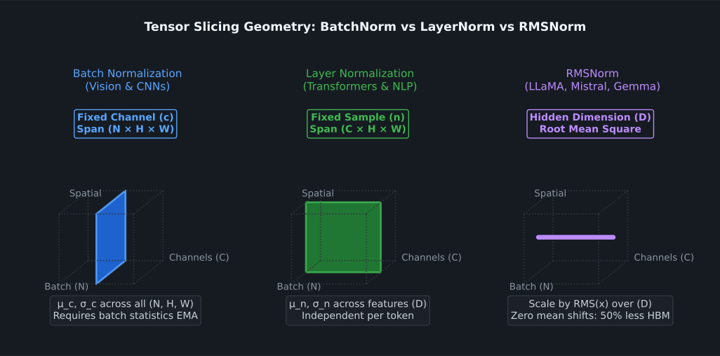
3. Layer Normalization & RMSNorm (The Transformer Era)
While Batch Normalization works brilliantly for fixed-size vision inputs, it fails on sequence data (text and audio) and small batch sizes: - Variable sequence lengths create varying batch sizes across time. - On small batch sizes ($N < 8$), mini-batch statistics become noisy and chaotic.
Layer Normalization (LayerNorm)
Ba, Kiros, & Hinton (2016) proposed normalizing across the feature channels of a single sample, completely independent of other samples in the batch:
$$\mu_i = \frac{1}{D} \sum_{j=1}^D x_{ij}, \quad \sigma_i^2 = \frac{1}{D} \sum_{j=1}^D (x_{ij} - \mu_i)^2$$
$$y_{ij} = \gamma_j \left( \frac{x_{ij} - \mu_i}{\sqrt{\sigma_i^2 + \epsilon}} \right) + \beta_j$$
Because statistics are computed independently per token, LayerNorm behaves identically during training and inference.
RMSNorm: Streamlined Normalization for Modern LLMs
Zhang & Sennrich (2019) demonstrated that the primary benefit of LayerNorm is not mean-centering, but scaling by activation magnitude.
Root Mean Square Normalization (RMSNorm) eliminates mean-centering entirely, reducing memory transfers by $50\%$ on GPU hardware:
$$\text{RMS}(\mathbf{x}_i) = \sqrt{\frac{1}{D} \sum_{j=1}^D x_{ij}^2 + \epsilon}$$
$$\mathbf{y}_i = \frac{\mathbf{x}_i}{\text{RMS}(\mathbf{x}_i)} \odot \gamma$$
Concrete Comparative Worked Example: The Normalization Trio
Consider a mini-batch of $N = 2$ tokens with $D = 3$ feature dimensions:
$$\mathbf{X} = \begin{bmatrix} 2.0 & 4.0 & 6.0 \\ 4.0 & 2.0 & 0.0 \end{bmatrix}$$
Let us compute the normalized output for Token 0 under each method ($\epsilon = 0, \gamma = 1, \beta = 0$):
Batch Normalization (Column-wise across Batch N)
Computes statistics independently for each feature channel across all samples in the mini-batch:
Layer Normalization (Row-wise across Features D)
Computes statistics independently for each token across its embedding vector ($[2.0, 4.0, 6.0]$):
RMSNorm (Root Mean Square Scaling without Mean Centering)
Scales token activations by their quadratic root mean square without subtracting the mean:
Hardware Implication: - LayerNorm requires 2 separate reduction loops (pass 1 to compute $\mu$, pass 2 to compute $\sigma^2$). - RMSNorm requires only 1 reduction pass (accumulating $x_j^2$), saving half the memory read traffic on GPU HBM!
4. Regularization: Preventing Overfitting
A deep network has enough parameter capacity to memorize the training data pixel-by-pixel. Regularization prevents memorization and forces the model to learn generalizable features.
Dropout & Inverted Dropout Derivation
Srivastava et al. (2014) introduced Dropout. During training, each neuron is independently zeroed out with probability $p$ (typically $p = 0.1$ to $0.5$):
$$r_j \sim \text{Bernoulli}(1 - p)$$
$$\tilde{x}_j = \frac{r_j}{1 - p} \cdot x_j$$
Why Divide by $1 - p$? (Zero Hidden Assumptions Proof)
Let us prove why the scaling factor $\frac{1}{1 - p}$ is required during training:
- The indicator variable $r_j \in \{0, 1\}$ takes value $1$ with probability $1 - p$ and value $0$ with probability $p$.
- The expectation of $r_j$ is: $$\mathbb{E}[r_j] = 1 \cdot (1 - p) + 0 \cdot p = 1 - p$$
- Taking the expected value of the scaled activation $\tilde{x}_j$: $$\mathbb{E}[\tilde{x}_j] = \mathbb{E}\left[ \frac{r_j}{1 - p} x_j \right] = \frac{x_j}{1 - p} \mathbb{E}[r_j] = \frac{x_j}{1 - p} (1 - p) = x_j$$
Because $\mathbb{E}[\tilde{x}_j] = x_j$, the expected magnitude of activations is mathematically identical between training mode and evaluation mode. At test time, dropout is simply bypassed with zero modifications to weights!
The factor $\frac{1}{1 - p}$ is Inverted Dropout scaling, ensuring the expected value remains identical during training and evaluation:
$$\mathbb{E}[\tilde{x}_j] = \frac{(1 - p) \cdot x_j}{1 - p} = x_j$$
Why Dropout works: No single neuron can rely on the presence of another specific neuron. The network is forced to learn redundant, robust feature representations across multiple independent pathways.
5. Prototypical NetCL Implementation
NetCL provides fully differentiable implementations of BatchNorm2d, Dropout, and RMSNorm:
import numpy as np
import netcl.autograd as ag
import netcl.nn as nn
from netcl.core.device import manager
from netcl.core.tensor import Tensor

q = manager.default("auto").queue

# 1. Vision Layer: Conv2d + BatchNorm2d + ReLU
conv = nn.Conv2d(q, in_channels=16, out_channels=32, kernel_size=3, padding=1)
bn = nn.BatchNorm2d(q, num_features=32)
relu = nn.ReLU()
dropout = nn.Dropout(p=0.2)

# 2. Input batch: (Batch=8, Channels=16, Height=28, Width=28)
x_raw = Tensor.from_host(q, np.random.randn(8, 16, 28, 28).astype(np.float32))

with ag.Tape() as tape:
    x_node = ag.tensor(x_raw)
    h = conv(x_node)
    h = bn(h)          # Normalizes across batch and spatial dimensions
    h = relu(h)
    h = dropout(h)     # Inverted dropout on GPU

print(f"Normalized Output Shape: {h.value.shape}")
assert h.value.shape == (8, 32, 28, 28)

# 3. Switching to evaluation mode
bn.eval()
dropout.eval()
print("BatchNorm running stats locked. Dropout disabled for inference.")
Related Documentation
- Concepts: BatchNorm: OpenCL kernel implementation of parallel channel reductions.
- NN API Reference: Full method signatures for
BatchNorm2d,Dropout, and layers. - Concepts: Transformer: Implementation of RMSNorm in sequence decoder blocks.
Next Steps in the Curriculum
Now that you know how to build and stabilize deep representations, how do we process natural language and sequences using the attention mechanism?
Proceed to Chapter 7: Tokens & Attention to learn about Byte-Pair Encoding (BPE), embedding tables, and Scaled Dot-Product Attention.