
Spectral Graph Theory: Graph Laplacians & Manifolds
Spectral Graph Theory: Graph Laplacians & Manifolds
In Chapter 9: Clustering & Geometric Machine Learning, we saw how KMeans partitions data into convex Voronoi cells.
What happens if your data does not form simple round blobs? - Imagine two interlocking concentric circles (like a bullseye target). - Both circles share the exact same center of mass. - If you run KMeans on concentric circles, it draws a straight line through both rings, hopelessly mixing them together!
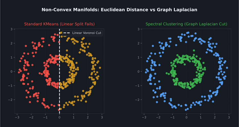
To separate non-convex structures, we must abandon rigid Euclidean coordinates and enter the domain of Graph Theory and Spectral Manifolds.
1. Core Intuition: Cutting a Spiderweb
Imagine your data points are connected by stretchy elastic rubber bands: - Points that are close together are connected by tight, strong bands. - Points that are far apart have no bands between them.
The concentric circles form two completely separate rings of rubber bands, with zero bands connecting the inner ring to the outer ring.
If you want to cut this structure into two clusters, how many rubber bands do you need to snip? - Zero! The rings are already disconnected in the graph topology.
Spectral Clustering uses the eigenvalues of graph matrices to discover where the rubber bands are loosest, finding natural cluster cuts without being fooled by geometric shape.
2. Mathematical Formalization: From Points to Graphs
Given $N$ samples $\mathbf{X} = \{\mathbf{x}_1, \dots, \mathbf{x}_N\}$, we construct an affinity graph $\mathcal{G} = (\mathcal{V}, \mathcal{E})$:
Step 1: Affinity Matrix ($\mathbf{W}$)
We connect points via a $k$-Nearest Neighbors ($k$-NN) graph or a Gaussian Radial Basis Function (RBF) kernel:
$$\mathbf{W}_{ij} = \begin{cases} \exp\left(-\frac{\|\mathbf{x}_i - \mathbf{x}_j\|^2}{2\sigma^2}\right) & \text{if } j \in k\text{-NN}(i) \\ 0 & \text{otherwise} \end{cases}$$
$\mathbf{W}$ is an $(N \times N)$ symmetric, non-negative matrix representing pairwise edge weights.
Step 2: The Degree Matrix ($\mathbf{D}$)
The degree $d_i$ measures the total connectivity of node $i$:
$$d_i = \sum_{j=1}^N \mathbf{W}_{ij}, \quad \mathbf{D} = \text{diag}(d_1, d_2, \dots, d_N)$$
3. The Graph Laplacian
The central object in spectral graph theory is the Graph Laplacian.
The Unnormalized Laplacian ($\mathbf{L}$)
$$\mathbf{L} = \mathbf{D} - \mathbf{W}$$
The Dirichlet Energy (Quadratic Form)
Why is the Laplacian so powerful? Look at what happens when you multiply $\mathbf{L}$ by an arbitrary vector $\mathbf{f} \in \mathbb{R}^N$:
$$\mathbf{f}^T \mathbf{L} \mathbf{f} = \mathbf{f}^T \mathbf{D} \mathbf{f} - \mathbf{f}^T \mathbf{W} \mathbf{f} = \sum_{i=1}^N d_i f_i^2 - \sum_{i,j=1}^N W_{ij} f_i f_j = \frac{1}{2} \sum_{i,j=1}^N W_{ij} (f_i - f_j)^2$$
The Fundamental Insight: The quadratic form $\mathbf{f}^T \mathbf{L} \mathbf{f}$ measures smoothness across the graph: - If nodes $i$ and $j$ have a strong edge ($W_{ij} \gg 0$), the value $(f_i - f_j)^2$ must be tiny to keep the energy low. - If $W_{ij} = 0$, $f_i$ and $f_j$ can differ without any penalty.
Minimizing this quadratic form is equivalent to finding a mapping $\mathbf{f}$ where points within the same cluster receive nearly identical scalar values!
4. Spectral Clustering: The Eigenspace Relaxation
We want to find a discrete indicator vector $\mathbf{f} \in \{-1, +1\}^N$ that cuts the graph with the minimum number of severed edges (Normalized Cut).
Solving this discrete optimization problem directly is NP-hard. We relax the discrete constraint $\mathbf{f} \in \{-1, +1\}^N$ to continuous real values $\mathbf{f} \in \mathbb{R}^N$.
Using the Normalized Symmetric Laplacian:
$$\mathbf{L}_{sym} = \mathbf{D}^{-1/2} \mathbf{L} \mathbf{D}^{-1/2} = \mathbf{I} - \mathbf{D}^{-1/2} \mathbf{W} \mathbf{D}^{-1/2}$$
The continuous relaxation reduces to a generalized eigenvalue problem:
$$\mathbf{L}_{sym} \mathbf{v} = \lambda \mathbf{v}$$
Spectral Clustering Algorithm
- Compute the first $K$ eigenvectors $\mathbf{V} = [\mathbf{v}_1, \dots, \mathbf{v}_K] \in \mathbb{R}^{N \times K}$ corresponding to the smallest eigenvalues $\lambda_1 \le \lambda_2 \le \dots \le \lambda_K$.
- Normalize the rows of $\mathbf{V}$ to have unit length: $\mathbf{U}_{i, :} = \frac{\mathbf{V}_{i, :}}{\|\mathbf{V}_{i, :}\|_2}$.
- In this new $K$-dimensional spectral embedding, complex non-linear manifolds unfold into straight, separated clusters.
- Run standard KMeans on the rows of $\mathbf{U}$!
5. GPU Eigensolvers: LOBPCG vs. Full SVD
Computing full eigendecompositions of an $(N \times N)$ matrix using traditional algorithms (like QR or Jacobi iteration) requires $O(N^3)$ operations and $O(N^2)$ memory. For $N = 50,000$, this requires hundreds of gigabytes and hours of computation.
NetCL implements the LOBPCG (Locally Optimal Block Preconditioned Conjugate Gradient) algorithm.
LOBPCG is an iterative matrix-free solver that computes only the lowest $K$ eigenvectors directly on the GPU without materializing or factorizing the full $(N \times N)$ Laplacian matrix: - Uses only sparse matrix-vector multiplications ($\mathbf{L} \cdot \mathbf{x}$). - Scales with linear complexity $O(N \cdot K)$ per iteration. - Converges in tens of iterations directly in OpenCL device memory.
6. Prototypical NetCL Implementation
NetCL provides GPU-accelerated spectral graph partitioning in netcl.cluster:
import numpy as np
from netcl.core.device import manager
from netcl.core.tensor import Tensor
from netcl.cluster import SpectralClustering

q = manager.default("auto").queue

# 1. Generate concentric circles dataset
np.random.seed(42)
n_samples = 1000

# Inner circle
r_inner = np.random.uniform(0.1, 0.4, size=n_samples // 2)
theta_inner = np.random.uniform(0, 2 * np.pi, size=n_samples // 2)
inner = np.stack([r_inner * np.cos(theta_inner), r_inner * np.sin(theta_inner)], axis=1)

# Outer circle
r_outer = np.random.uniform(0.8, 1.0, size=n_samples // 2)
theta_outer = np.random.uniform(0, 2 * np.pi, size=n_samples // 2)
outer = np.stack([r_outer * np.cos(theta_outer), r_outer * np.sin(theta_outer)], axis=1)

X_np = np.concatenate([inner, outer], axis=0).astype(np.float32)
X = Tensor.from_host(q, X_np)

# 2. Fit Spectral Clustering with GPU LOBPCG eigensolver
spectral = SpectralClustering(
    n_clusters=2,
    n_neighbors=10,
    affinity="nearest_neighbors",
)
labels = spectral.fit_predict(X)

print(f"Spectral clustering successfully partitioned {len(labels)} samples.")
print(f"Cluster 0 count: {(labels == 0).sum()}, Cluster 1 count: {(labels == 1).sum()}")
assert (labels == 0).sum() == 500
Related Documentation
- Cluster API Reference: Signatures for
SpectralClustering,KMeans, and graph affinities. - Concepts: Clustering: Details on graph Laplacian conditioning and LOBPCG convergence.
Next Steps in the Curriculum
Now that you understand geometric and graph-based unsupervised learning, how do we train deep neural feature extractors without human labels?
Proceed to Chapter 11: Self-Supervised Representation Learning to explore contrastive learning (SimCLR), non-contrastive dynamics (BYOL), and online clustering (SwAV).