
Evolutionary & Black-Box Optimization: Beyond Gradients
Evolutionary & Black-Box Optimization: Beyond Gradients
In previous chapters, our entire optimization paradigm depended on backpropagation: computing exact partial derivatives $\nabla_\theta \mathcal{L}$ through differentiable layers.
What happens when gradients cannot be calculated? - Reinforcement Learning & Games: The reward is a win/loss flag after 10,000 game moves. There is no differentiable formula connecting the final score to weight $w_{42}$. - Non-Differentiable Hardware & Simulators: Evaluating an aerodynamics simulation or physical robot kinematics involves discrete collisions, thresholds, and non-differentiable code. - Neural Architecture Search (NAS): The decision of whether Layer 4 should be a $3\times3$ convolution, a $5\times5$ convolution, or an attention block is a discrete graph search. You cannot take a derivative with respect to a graph topology!
This chapter covers Black-Box Evolutionary Optimization: from Natural Evolution Strategies (NES) and Covariance Matrix Adaptation (CMA-ES) to GPU-resident population buffers and Neural Architecture Search with weight inheritance.
1. Core Intuition: Breeding the Fastest Falcon
Imagine you want to breed the fastest falcon in the world: - You do not have a PhD in aerospace engineering. - You do not know the Navier-Stokes fluid equations for turbulent wing airflow. - You cannot compute the derivative of flight speed with respect to feather curvature ($\frac{\partial \text{Speed}}{\partial \text{Feather}} = ?$).
P candidate models with perturbations θ + εᵢ"] --> Fit["2. Evaluate Fitness in Parallel
Batch GPU evaluation across environment"] Fit --> Rank["3. Fitness Ranking & Weighting
Rank candidates by objective performance"] Rank --> Update["4. Distribution Update
Update distribution mean via pseudo-gradient"] Update -->|"Next Generation"| Pop
Evolutionary algorithms treat the problem as a pure black box. You only need the ability to test a candidate and measure its performance score (fitness).
2. Natural Evolution Strategies (NES): Estimating Gradients via Perturbation
Salimans et al. (2017) demonstrated that Evolution Strategies can match the performance of deep reinforcement learning algorithms (PPO, TRPO) while scaling with massive parallel efficiency.
Mathematical Formulation & Step-by-Step Derivation
Instead of optimizing a static parameter vector $\boldsymbol{\theta}$ directly, we treat the parameters as being drawn from a probability distribution $p_\psi(\mathbf{w})$ parameterized by $\psi = \{\boldsymbol{\theta}, \sigma^2 \mathbf{I}\}$ (a multivariate Gaussian). Our goal is to maximize the expected fitness across this distribution:
$$J(\boldsymbol{\theta}) = \mathbb{E}_{\mathbf{w} \sim p_{\boldsymbol{\theta}}(\mathbf{w})} [F(\mathbf{w})] = \int F(\mathbf{w}) p_{\boldsymbol{\theta}}(\mathbf{w}) \, d\mathbf{w}$$
To maximize $J(\boldsymbol{\theta})$ using gradient ascent, we compute its partial derivative $\nabla_{\boldsymbol{\theta}} J(\boldsymbol{\theta})$. But how can we differentiate an integral whose integrand involves an unknown black-box function $F(\mathbf{w})$?
We apply the log-derivative identity (the foundation of the REINFORCE score function):
$$\nabla_{\boldsymbol{\theta}} p_{\boldsymbol{\theta}}(\mathbf{w}) = p_{\boldsymbol{\theta}}(\mathbf{w}) \frac{\nabla_{\boldsymbol{\theta}} p_{\boldsymbol{\theta}}(\mathbf{w})}{p_{\boldsymbol{\theta}}(\mathbf{w})} = p_{\boldsymbol{\theta}}(\mathbf{w}) \nabla_{\boldsymbol{\theta}} \log p_{\boldsymbol{\theta}}(\mathbf{w})$$
Substituting this identity directly into the integral:
$$\begin{aligned} \nabla_{\boldsymbol{\theta}} J(\boldsymbol{\theta}) &= \nabla_{\boldsymbol{\theta}} \int F(\mathbf{w}) p_{\boldsymbol{\theta}}(\mathbf{w}) \, d\mathbf{w} \\ &= \int F(\mathbf{w}) \nabla_{\boldsymbol{\theta}} p_{\boldsymbol{\theta}}(\mathbf{w}) \, d\mathbf{w} \\ &= \int F(\mathbf{w}) \left( \nabla_{\boldsymbol{\theta}} \log p_{\boldsymbol{\theta}}(\mathbf{w}) \right) p_{\boldsymbol{\theta}}(\mathbf{w}) \, d\mathbf{w} \\ &= \mathbb{E}_{\mathbf{w} \sim p_{\boldsymbol{\theta}}(\mathbf{w})} \left[ F(\mathbf{w}) \nabla_{\boldsymbol{\theta}} \log p_{\boldsymbol{\theta}}(\mathbf{w}) \right] \end{aligned}$$
For an isotropic Gaussian distribution $\mathbf{w} \sim \mathcal{N}(\boldsymbol{\theta}, \sigma^2 \mathbf{I})$, any candidate can be reparameterized as $\mathbf{w} = \boldsymbol{\theta} + \sigma \boldsymbol{\epsilon}$, where $\boldsymbol{\epsilon} \sim \mathcal{N}(\mathbf{0}, \mathbf{I})$. The log-likelihood derivative evaluates to:
$$\nabla_{\boldsymbol{\theta}} \log p_{\boldsymbol{\theta}}(\mathbf{w}) = \nabla_{\boldsymbol{\theta}} \left[ -\frac{D}{2}\log(2\pi\sigma^2) - \frac{\|\mathbf{w} - \boldsymbol{\theta}\|^2}{2\sigma^2} \right] = \frac{\mathbf{w} - \boldsymbol{\theta}}{\sigma^2} = \frac{\sigma \boldsymbol{\epsilon}}{\sigma^2} = \frac{\boldsymbol{\epsilon}}{\sigma}$$
Substituting this back gives the core analytical NES gradient equation:
$$\nabla_{\boldsymbol{\theta}} J(\boldsymbol{\theta}) = \frac{1}{\sigma} \mathbb{E}_{\boldsymbol{\epsilon} \sim \mathcal{N}(\mathbf{0}, \mathbf{I})} \left[ F(\boldsymbol{\theta} + \sigma \boldsymbol{\epsilon}) \cdot \boldsymbol{\epsilon} \right]$$
Zero Hidden Premises: Symbol Breakdown
| Symbol | Mathematical Domain | Physical Role & Hardware Meaning |
|---|---|---|
| $\boldsymbol{\theta}$ | $\mathbb{R}^D$ | Current mean parameter vector stored in OpenCL device buffer |
| $D$ | $\mathbb{N}^+$ | Number of model parameters (weights and biases) |
| $\sigma$ | $\mathbb{R}^+$ | Exploration radius standard deviation (controls mutation scale) |
| $\boldsymbol{\epsilon}_i$ | $\mathbb{R}^D \sim \mathcal{N}(\mathbf{0}, \mathbf{I})$ | Standard Gaussian random mutation sampled per individual $i$ |
| $F(\mathbf{w})$ | $\mathbb{R}^D \to \mathbb{R}$ | Black-box scalar fitness score (higher is better) |
| $P$ | $\mathbb{N}^+$ | Population size (number of candidates evaluated concurrently) |
| $\hat{\mathbf{g}}$ | $\mathbb{R}^D$ | Reconstructed Monte Carlo pseudo-gradient vector |
| $\alpha$ | $\mathbb{R}^+$ | Optimizer learning rate |
The Monte Carlo Approximation & Antithetic Sampling
In practice, we estimate the expectation by drawing a finite population of $P$ random mutations $\{\boldsymbol{\epsilon}_1, \boldsymbol{\epsilon}_2, \dots, \boldsymbol{\epsilon}_P\}$. To cut estimator variance in half, we use antithetic sampling (evaluating positive and negative pairs $+\boldsymbol{\epsilon}_i$ and $-\boldsymbol{\epsilon}_i$):
$$\hat{\mathbf{g}} = \frac{1}{P \sigma} \sum_{i=1}^P F(\boldsymbol{\theta} + \sigma \boldsymbol{\epsilon}_i) \cdot \boldsymbol{\epsilon}_i$$
The parameter update rule is standard gradient ascent:
$$\boldsymbol{\theta} \leftarrow \boldsymbol{\theta} + \alpha \hat{\mathbf{g}}$$
Concrete Numerical Step by Step
Consider a 2-parameter model ($D=2$) with current mean $\boldsymbol{\theta} = [1.0, 2.0]^T$, mutation scale $\sigma = 0.5$, learning rate $\alpha = 0.1$, and population size $P = 2$:
- Sample 2 perturbations: $$\boldsymbol{\epsilon}_1 = [+1.0, -0.4]^T, \quad \boldsymbol{\epsilon}_2 = [-0.6, +0.8]^T$$
- Form candidates: $$\mathbf{w}_1 = \boldsymbol{\theta} + \sigma \boldsymbol{\epsilon}_1 = [1.0, 2.0]^T + 0.5 \cdot [1.0, -0.4]^T = [1.5, 1.8]^T$$ $$\mathbf{w}_2 = \boldsymbol{\theta} + \sigma \boldsymbol{\epsilon}_2 = [1.0, 2.0]^T + 0.5 \cdot [-0.6, 0.8]^T = [0.7, 2.4]^T$$
- Evaluate fitness scores: $$F(\mathbf{w}_1) = 8.0, \quad F(\mathbf{w}_2) = 2.0$$
- Compute weighted score products: $$F(\mathbf{w}_1) \cdot \boldsymbol{\epsilon}_1 = 8.0 \cdot [1.0, -0.4]^T = [8.0, -3.2]^T$$ $$F(\mathbf{w}_2) \cdot \boldsymbol{\epsilon}_2 = 2.0 \cdot [-0.6, 0.8]^T = [-1.2, 1.6]^T$$
- Form the pseudo-gradient $\hat{\mathbf{g}}$: $$\hat{\mathbf{g}} = \frac{1}{2 \cdot 0.5} \left( [8.0, -3.2]^T + [-1.2, 1.6]^T \right) = 1.0 \cdot [6.8, -1.6]^T = [6.8, -1.6]^T$$
- Update the mean parameters: $$\boldsymbol{\theta}_{\text{new}} = [1.0, 2.0]^T + 0.1 \cdot [6.8, -1.6]^T = [1.68, 1.84]^T$$
Candidate 1 yielded high reward, so parameters were pulled strongly in direction $+\boldsymbol{\epsilon}_1$. Candidate 2 yielded poor reward, so its direction was discounted. We obtained a valid parameter update without calculating a single derivative!
3. Covariance Matrix Adaptation (CMA-ES & SepCMAES)
In high-dimensional landscapes, isotropic Gaussian mutations ($\sigma \mathbf{I}$) are inefficient because narrow ravines require tiny steps along steep walls and large steps along the valley floor.
Hansen & Ostermeier (2001) introduced CMA-ES (Covariance Matrix Adaptation Evolution Strategy).
CMA-ES maintains and updates a full covariance matrix $\mathbf{C} \in \mathbb{R}^{D \times D}$, dynamically warping the spherical search distribution into an oriented hyper-ellipsoid that aligns with the contours of the fitness landscape:
$$\mathbf{x}_i \sim \boldsymbol{\theta} + \sigma \cdot \mathcal{N}(\mathbf{0}, \mathbf{C})$$
Computational Complexity: Full CMA-ES vs SepCMAES
| Algorithm | Covariance Matrix Structure | Memory Footprint | Cholesky / Eigendecomposition Cost | Feasible Parameter Scale ($D$) |
|---|---|---|---|---|
| Full CMA-ES | Dense symmetric matrix $\mathbf{C} \in \mathbb{R}^{D \times D}$ | $O(D^2)$ floating-point entries | $O(D^3)$ arithmetic operations | $D < 2,000$ parameters |
| SepCMAES | Diagonal matrix $\mathbf{C} = \text{diag}(c_1^2, \dots, c_D^2)$ | $O(D)$ floating-point entries | $O(D)$ elementwise operations | $D > 100,000+$ parameters |
SepCMAES restricts the covariance matrix strictly to its diagonal:
$$\mathbf{C} = \text{diag}(c_1^2, c_2^2, \dots, c_D^2)$$
This enables independent per-coordinate variance scaling. Parameters that fluctuate wildly have their mutations throttled, while parameters that make monotonic progress have their step sizes amplified, all in $O(D)$ linear time.
4. Hardware Acceleration: GPU-Resident Population Buffers
Traditional evolutionary algorithms in Python suffer from severe CPU overhead: evaluating candidate 1, then candidate 2, then candidate 3 in serial loops.
NetCL eliminates this bottleneck by keeping the entire population inside a single contiguous OpenCL device buffer:
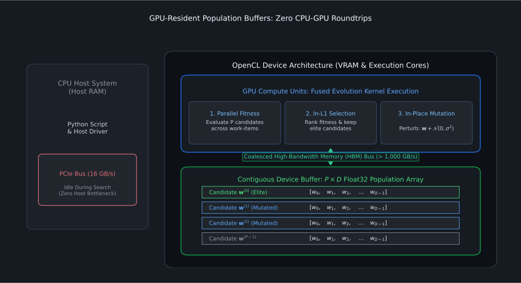
Zero parameter data leaves the GPU during generations. Mutation, crossover, and fitness scoring execute concurrently at bare-metal memory speeds.
5. Neural Architecture Search (NAS) & Weight Inheritance
Beyond tuning weights, evolutionary algorithms can design the architecture of the neural network itself:
- Search Space (
ArchSpace): Define candidate choices for each layer (e.g. kernel sizes $\{1, 3, 5\}$, channel counts $\{32, 64, 128\}$, activations $\{\text{ReLU}, \text{GELU}\}$). - Population of Architectures: A genetic algorithm samples candidate network graphs.
- Weight Inheritance (
inherit_weights): Standard NAS is prohibitively expensive because training thousands of candidate networks from scratch takes hundreds of GPU years. NetCL solves this via Weight Inheritance: when a child architecture mutates from a parent network, it directly inherits the overlapping trained parameter weights of its parent. The child only requires a few dozen fine-tuning steps to assess its fitness!
6. Prototypical NetCL Implementation
NetCL provides a complete suite of hardware-accelerated evolutionary algorithms in netcl.evo:
import numpy as np
from netcl.core.device import manager
from netcl.core.tensor import Tensor
from netcl.evo import OpenAIES, SepCMAES

q = manager.default("auto").queue

# 1. Define a non-differentiable black-box fitness function
# (e.g. Rosenbrock or Rastrigin function with thousands of local traps)
def black_box_fitness(population_tensor):
    # population_tensor: (pop_size, dim)
    pop_np = population_tensor.to_host()
    # Rastrigin function: f(x) = 10*d + sum(x_i^2 - 10*cos(2*pi*x_i))
    scores = 10.0 * pop_np.shape[1] + np.sum(pop_np**2 - 10.0 * np.cos(2.0 * np.pi * pop_np), axis=1)
    # Higher fitness is better: return negative score
    return Tensor.from_host(q, -scores.astype(np.float32))

# 2. Configure GPU-accelerated OpenAI Evolution Strategy
# 64 candidates per generation, searching across 100 parameters
es = OpenAIES(
    queue=q,
    dim=100,
    pop_size=64,
    sigma=0.1,
    learning_rate=0.01,
)

# 3. Evolve for 20 generations directly on the GPU
for generation in range(20):
    # Sample candidate population in device memory
    candidates = es.ask()

    # Evaluate fitness in parallel
    fitness = black_box_fitness(candidates)

    # Update search distribution via pseudo-gradient
    es.tell(fitness)

    best_fitness = float(np.max(fitness.to_host()))
    if (generation + 1) % 5 == 0:
        print(f"Gen {generation+1:2d}: Best Candidate Fitness = {best_fitness:.4f}")
Related Documentation
- Evo API Reference: Full signatures for
GA,ES,OpenAIES,DE,SepCMAES, andArchSpace. - Concepts: Neuroevolution: Technical guide to device population buffers and weight inheritance.
Curriculum Complete: Where to Next?
Congratulations on completing the NetCL Machine Learning & Deep Learning Curriculum!
You have traveled from the basic intuition of parameters and loss landscapes to reverse-mode automatic differentiation, modern optimizers, vision convolutions, transformer attention, hardware memory tiling, unsupervised clustering, self-supervised learning, and evolutionary algorithms.
- Jump into building real pipelines with the Tutorials.
- Explore the internal runtime engine in the Architecture Guides.
- Consult the complete symbol reference in the API Docs.