Self-Supervised Learning: Representations Without Human Labels

Supervised deep learning has a crippling limitation: it requires millions of manually annotated labels. Annotating medical scans, seismic data, or video streams costs millions of dollars and thousands of human hours.

Self-Supervised Learning (SSL) eliminates the human in the loop. By designing pretext tasks from the raw data itself, models learn rich, generalizable visual and semantic representations before a single human label is ever seen.

This chapter covers the three foundational pillars of modern SSL: Contrastive Learning (SimCLR, InfoNCE), Non-Contrastive Learning (BYOL, stop-gradients), and Online Cluster Assignment (SwAV, Sinkhorn transport).

1. Core Intuition: Recognizing Your Dog

Imagine your golden retriever: - You see your dog in bright morning sunlight. - You see your dog at dusk in the pouring rain. - You see your dog wearing a goofy birthday hat.

To your eyes, the raw pixel values are completely different (dark vs bright, blurry vs sharp). Yet your brain instantly knows: this is the exact same dog.

Self-supervised learning trains neural networks to have this exact intuition: 1. Take an unlabelled image $x$. 2. Create two distorted copies (views) $\tilde{x}_1$ and $\tilde{x}_2$ using random cropping, color jitter, and blur. 3. Pass both views through an encoder network to get embeddings $z_1$ and $z_2$. 4. Train the network so that the embedding of view 1 is as close as possible to the embedding of view 2, while remaining distinct from all other images in the dataset!

2. Contrastive Learning: SimCLR & The InfoNCE Loss

Chen et al. (2020) formalized this paradigm in SimCLR.

Positive vs. Negative Pairs

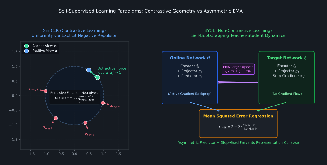
For a mini-batch of $N$ images, we generate $2N$ augmented views. - Positive Pair: Two augmented views $(\tilde{x}_i, \tilde{x}_j)$ originating from the same source image. - Negative Pairs: All other $2(N - 1)$ views in the batch, which originate from different source images.

The InfoNCE Loss (Noise-Contrastive Estimation)

We define the normalized temperature-scaled cosine similarity between embeddings:

$$\text{sim}(\mathbf{u}, \mathbf{v}) = \frac{\mathbf{u}^T \mathbf{v}}{\|\mathbf{u}\|_2 \|\mathbf{v}\|_2}$$

The loss function for a positive pair $(i, j)$ is:

$$\mathcal{L}_{i, j} = -\log \frac{\exp(\text{sim}(\mathbf{z}_i, \mathbf{z}_j) / \tau)}{\sum_{k=1}^{2N} \mathbb{I}_{[k \ne i]} \exp(\text{sim}(\mathbf{z}_i, \mathbf{z}_k) / \tau)}$$

Where $\tau > 0$ is a temperature hyperparameter (typically $\tau = 0.07$ to $0.1$).

The Geometric Dual: Alignment and Uniformity

Wang & Isola (2020) proved that optimizing InfoNCE simultaneously achieves two geometric objectives on the unit hypersphere: 1. Alignment (Numerator): Positive pairs pull together. Augmented views of the same object map to nearby points on the sphere. 2. Uniformity (Denominator): Negative pairs push apart. Features repel each other, distributing information uniformly across the entire hypersphere to maximize entropy.

3. The Representation Collapse Trap & Non-Contrastive Learning

Why do we need negative pairs in SimCLR?

What happens if we remove the denominator and simply minimize the distance between positive views:

$$\mathcal{L} = \|\mathbf{z}_1 - \mathbf{z}_2\|^2$$

The network quickly discovers a trivial mathematical cheat: Complete Representation Collapse.

If the encoder weights are set such that the network outputs a constant vector $\mathbf{z} = [1, 0, 0, \dots, 0]$ for every single image in the universe, then $\|\mathbf{z}_1 - \mathbf{z}_2\|^2 = 0$ perfectly! The loss is zero, but the representations are entirely useless.

Negative pairs in SimCLR prevent collapse by forcing different images to produce different vectors.

Non-Contrastive Learning: BYOL (Bootstrap Your Own Latent)

Can we train without negative pairs at all?

Grill et al. (2020) introduced BYOL, demonstrating that an asymmetric architecture with an Exponential Moving Average (EMA) teacher and a stop-gradient operator completely prevents collapse without negative pairs:

1. The Online Network $(\theta)$ receives view 1 and predicts the representation of view 2.
2. The Target Network $(\xi)$ receives view 2. Its weights are an EMA of past online weights and receive zero backpropagation gradients (stop_gradient).
3. The asymmetry between the predictor and target network breaks the mathematical symmetry required for collapse, allowing stable self-supervised learning without large batch sizes.

4. Deep Clustering & Optimal Transport: SwAV

Caron et al. (2020) introduced SwAV (Swapping Assignments between Views), combining self-supervised learning with online clustering.

Instead of comparing every image to every other image in the batch, SwAV introduces $K$ learnable prototype vectors $\mathbf{C} = [\mathbf{c}_1, \dots, \mathbf{c}_K] \in \mathbb{R}^{D \times K}$.

1. Features $\mathbf{z}_1$ and $\mathbf{z}_2$ are mapped to soft cluster assignment codes $\mathbf{q}_1$ and $\mathbf{q}_2$.
2. To prevent the cluster assignment from collapsing (all images assigned to a single cluster), SwAV solves an Optimal Transport problem via the Sinkhorn-Knopp algorithm, enforcing an equal partition constraint across clusters.
3. The loss enforces swapped prediction: feature $\mathbf{z}_1$ must predict cluster code $\mathbf{q}_2$, and feature $\mathbf{z}_2$ must predict cluster code $\mathbf{q}_1$.

5. Prototypical NetCL Implementation

NetCL provides end-to-end self-supervised models and device-side view generation in netcl.ssl:

import numpy as np
import netcl.autograd as ag
import netcl.nn as nn
from netcl.core.device import manager
from netcl.core.tensor import Tensor
from netcl.ssl import SimCLR, BYOL

q = manager.default("auto").queue

# 1. Base convolutional backbone (e.g. ResNet-18 or small CNN)
backbone = nn.Sequential(
    nn.Conv2d(q, 3, 32, kernel_size=3, padding=1),
    nn.ReLU(),
    nn.Conv2d(q, 32, 64, kernel_size=3, padding=1),
    nn.ReLU(),
)

# 2. Wrap backbone with SimCLR self-supervised model
simclr = SimCLR(
    queue=q,
    backbone=backbone,
    feature_dim=64,
    proj_dim=32,
    temperature=0.1,
)

# 3. Simulate two augmented views of an unlabelled batch (B=16, C=3, H=32, W=32)
view1 = Tensor.from_host(q, np.random.randn(16, 3, 32, 32).astype(np.float32))
view2 = Tensor.from_host(q, np.random.randn(16, 3, 32, 32).astype(np.float32))

with ag.Tape() as tape:
    # Forward both views through projection head
    z1 = simclr.project(ag.tensor(view1))
    z2 = simclr.project(ag.tensor(view2))

    # Compute InfoNCE loss across positive and negative pairs
    loss = simclr.loss(z1, z2)

tape.backward(loss)
print(f"Self-Supervised InfoNCE Loss: {loss.value.to_host()[0]:.4f}")

Related Documentation

• SSL API Reference: Signatures for SimCLR, BYOL, SwAV, DINO, and evaluation probes (KNNMonitor).
• Concepts: Metric Losses: Triplet loss, Contrastive margin loss, and batch hard mining.
• Concepts: SSL: View generation and online linear probe validation.

Next Steps in the Curriculum

Every method we have studied so far relies on gradients $\nabla_\theta \mathcal{L}$. What happens when gradients cannot be computed (discrete code, physical robots, or neural architecture topology)?

Proceed to Chapter 12: Evolutionary & Black-Box Optimization to explore Natural Evolution Strategies (NES), CMA-ES, and Neural Architecture Search (NAS).