Clustering & Geometric Machine Learning

In previous chapters, every model relied on labeled supervision: we provided inputs $\mathbf{X}$ and known ground-truth targets $\mathbf{y}$.

In the real world, $99\%$ of data has no labels. You have a database of 10 million customer purchase histories, 50 million protein sequences, or 100 million sensor readings, and you need to discover the hidden natural structure within them.

This chapter covers the geometric foundations of unsupervised clustering: from Voronoi partitions and KMeans to the distance matrix GPU memory trap, fused distance-argmin execution, and optimal transport equipartition.

1. Core Intuition: Finding Star Constellations

Look up at the night sky. There are thousands of scattered white dots.

When looking at a scatter of unlabeled data points in space, human perception naturally groups points into clusters based on spatial proximity and density boundaries.

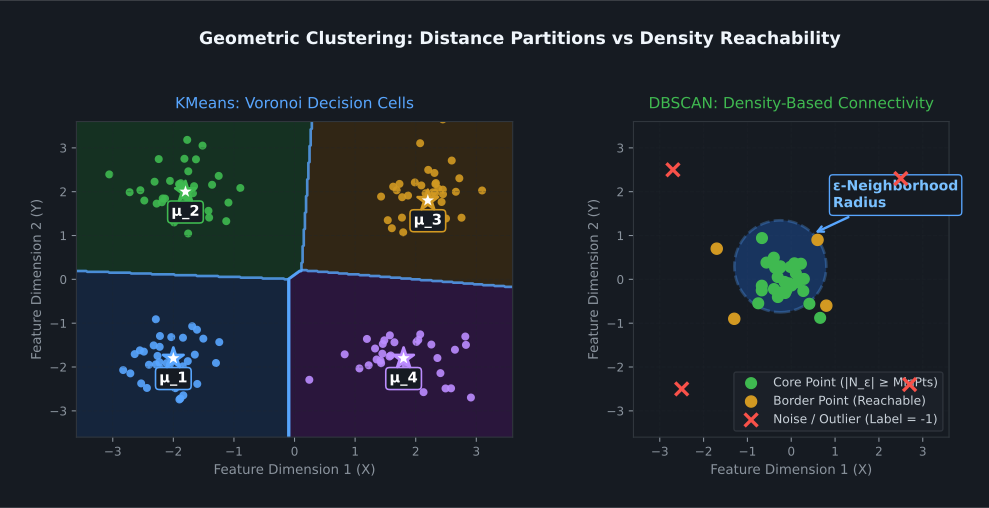
Unsupervised clustering formalizes this intuitive grouping: 1. Choose $K$ candidate cluster centers (centroids $\boldsymbol{\mu}_1, \dots, \boldsymbol{\mu}_K$). 2. Assign each point in the dataset to its closest centroid. 3. Move each centroid to the center of mass (mean) of the points assigned to it. 4. Repeat until the centroids stabilize.

2. Mathematical Formalization: KMeans & Voronoi Partitions

Given a dataset of $N$ points $\mathbf{X} = \{\mathbf{x}_1, \dots, \mathbf{x}_N\} \subset \mathbb{R}^D$, we seek to partition the data into $K$ disjoint subsets $S = \{S_1, \dots, S_K\}$.

The Objective: Within-Cluster Sum of Squares (WCSS)

We want to minimize the total squared Euclidean distance between every point and its assigned cluster centroid:

$$\mathcal{J}(S, \boldsymbol{\mu}) = \sum_{k=1}^K \sum_{\mathbf{x} \in S_k} \|\mathbf{x} - \boldsymbol{\mu}_k\|^2$$

Lloyd's Algorithm (Expectation-Maximization)

Lloyd (1982) demonstrated that this non-convex optimization problem converges monotonically to a local minimum via two alternating steps:

1. Assignment Step (E-Step): Assign each sample $\mathbf{x}_i$ to the nearest centroid, carving the space into Voronoi cells:

$$c_i = \arg\min_{k \in \{1, \dots, K\}} \|\mathbf{x}_i - \boldsymbol{\mu}_k\|^2$$

2. Update Step (M-Step): Recompute each centroid as the arithmetic mean of all points assigned to that Voronoi cell:

$$\boldsymbol{\mu}_k = \frac{1}{|S_k|} \sum_{i \in S_k} \mathbf{x}_i$$

3. The GPU Distance Matrix Memory Trap

On paper, the assignment step requires evaluating distances between all $N$ points and all $K$ centroids:

$$\mathbf{D}_{ik} = \|\mathbf{x}_i - \boldsymbol{\mu}_k\|^2 = \|\mathbf{x}_i\|^2 - 2 \mathbf{x}_i \cdot \boldsymbol{\mu}_k + \|\boldsymbol{\mu}_k\|^2$$

Standard high-level frameworks (like Scikit-learn or naive PyTorch) compute this by materializing the entire $(N \times K)$ distance matrix $\mathbf{D}$ in VRAM: - For $N = 500,000$ points and $K = 4,096$ clusters:

$$500,000 \times 4,096 \times 4 \text{ bytes} \approx 8.19 \text{ GB of VRAM}$$

Materializing this matrix crashes consumer GPUs with out-of-memory errors before a single iteration completes!

The NetCL Solution: Fused Distance-Argmin Kernel

NetCL avoids materializing the distance matrix entirely by fusing the distance calculation and the minimum search into a single OpenCL GPU kernel:

__kernel void fused_kmeans_assign(
    __global const float* restrict X,       // (N, D)
    __global const float* restrict centroids, // (K, D)
    __global int* restrict labels,          // (N,)
    const int N, const int D, const int K
) {
    int i = get_global_id(0);
    if (i >= N) return;

    float min_dist = 1e30f;
    int best_k = 0;

    // Scan all centroids entirely within local GPU registers
    for (int k = 0; k < K; k++) {
        float dist = 0.0f;
        for (int d = 0; d < D; d++) {
            float diff = X[i * D + d] - centroids[k * D + d];
            dist += diff * diff;
        }
        if (dist < min_dist) {
            min_dist = dist;
            best_k = k;
        }
    }
    labels[i] = best_k; // Only write the scalar integer index to VRAM!
}

Memory consumption drops from $O(N \cdot K)$ to $O(N)$. Instead of 8.2 GB, NetCL requires only 2 MB of memory, enabling clustering of millions of points on modest hardware.

4. Advanced Geometric Variants

Spherical KMeans (Cosine Similarity)

In natural language and representation learning, vector magnitude often represents word frequency or brightness rather than semantics.

Spherical KMeans projects all points and centroids onto the unit hypersphere $S^{D-1}$:

$$\tilde{\mathbf{x}} = \frac{\mathbf{x}}{\|\mathbf{x}\|_2}, \quad \tilde{\boldsymbol{\mu}} = \frac{\boldsymbol{\mu}}{\|\boldsymbol{\mu}\|_2}$$

Minimizing Euclidean distance on the sphere is equivalent to maximizing Cosine Similarity:

$$\arg\min_k \|\tilde{\mathbf{x}} - \tilde{\boldsymbol{\mu}}_k\|^2 \iff \arg\max_k (\tilde{\mathbf{x}} \cdot \tilde{\boldsymbol{\mu}}_k)$$

Balanced KMeans via Sinkhorn Optimal Transport

In standard KMeans, popular clusters can grow disproportionately large while other clusters become empty.

Balanced KMeans enforces an equipartition constraint: every cluster must contain exactly $\frac{N}{K}$ samples. This is solved via the Sinkhorn-Knopp algorithm, treating cluster assignment as an optimal transport problem between the empirical data distribution and uniform cluster priors.

5. Prototypical NetCL Implementation

NetCL provides a full suite of GPU-accelerated clustering algorithms in netcl.cluster:

import numpy as np
from netcl.core.device import manager
from netcl.core.tensor import Tensor
from netcl.cluster import KMeans, SphericalKMeans, BalancedKMeans

q = manager.default("auto").queue

# 1. Generate synthetic dataset: 10,000 samples in 32 dimensions
X_np = np.random.randn(10000, 32).astype(np.float32)
X = Tensor.from_host(q, X_np)

# 2. Standard GPU-Accelerated KMeans
kmeans = KMeans(n_clusters=16, max_iter=50, tol=1e-4)
kmeans.fit(X)

print(f"KMeans converged in {kmeans.n_iter_} iterations.")
print(f"Centroids shape: {kmeans.cluster_centers_.shape}")
assert kmeans.cluster_centers_.shape == (16, 32)

# 3. Predict cluster assignments for new data
labels = kmeans.predict(X)
print(f"Assigned labels shape: {labels.shape}")

Related Documentation

• Cluster API Reference: Full API documentation for KMeans, MiniBatchKMeans, BalancedKMeans, GaussianMixture, and DBSCAN.
• Concepts: Clustering: Technical guide to GPU memory bandwidth and convergence criteria.

Next Steps in the Curriculum

Standard KMeans assumes clusters are convex, spherical blobs in Euclidean space. What if the clusters form complex spirals or interconnected graph manifolds?

Proceed to Chapter 10: Spectral Graph Theory & Manifolds to learn about Graph Laplacians, eigenmaps, and LOBPCG eigensolvers.