
Hardware Realities & FlashAttention: Breaking the Memory Wall
Hardware Realities & FlashAttention: Breaking the Memory Wall
In Chapter 7: Tokens & Attention, we derived Scaled Dot-Product Attention:
$$\text{Attention}(\mathbf{Q}, \mathbf{K}, \mathbf{V}) = \text{softmax}\left(\frac{\mathbf{Q}\mathbf{K}^T}{\sqrt{d_k}}\right)\mathbf{V}$$
On paper, this formula is elegant. On physical GPU hardware, naive execution triggers an immediate crisis: - If sequence length $S = 16,384$ tokens, the attention matrix $\mathbf{A} \in \mathbb{R}^{S \times S}$ contains $268,435,456$ elements. - Storing this matrix across 32 attention heads in float32 requires 34 GB of VRAM for a single attention layer!
This chapter explains the physical memory hierarchy of modern GPUs, introduces the Roofline Model, and reveals how FlashAttention and KV-caching enable long-context models to execute on consumer hardware.
1. Core Intuition: The Kitchen Counter vs. The Basement Pantry
Imagine a master chef preparing a complex banquet: - The Kitchen Cutting Board (GPU Registers / Local SRAM): Extremely fast to grab ingredients from, but tiny. It can only hold 2 or 3 ingredients at a time. - The Basement Walk-in Pantry (VRAM / HBM): Massive storage holding 16 GB of supplies, but located down two flights of stairs. Every trip to the pantry takes several minutes.
Compute throughput: ~40 TFLOPs"] Local["On-Chip Local SRAM & Registers
~19 TB/s bandwidth · a few hundred KB capacity"] VRAM["Device VRAM / HBM Global Memory
~0.8 TB/s bandwidth · 8 GB to 24 GB capacity"] Cores -->|"Ultra-fast register access"| Local Local -->|"10x to 50x slower bus transfer"| VRAM
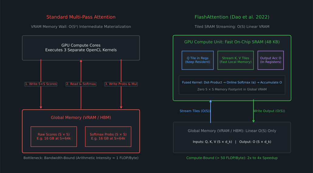
The Tragedy of Naive Attention: 1. The GPU reads $\mathbf{Q}$ and $\mathbf{K}$ from VRAM, computes $\mathbf{S} = \mathbf{Q}\mathbf{K}^T$, and walks down to the pantry to write the massive $S \times S$ matrix back to VRAM. 2. Then it reads that matrix back from VRAM, computes $\text{softmax}(\mathbf{S})$, and walks down to the pantry again to write the $S \times S$ probability matrix. 3. Then it reads that matrix back from VRAM a third time, multiplies it by $\mathbf{V}$, and writes the output.
The GPU compute cores spend $90\%$ of their time idling, waiting for bytes to trickle across the memory bus from VRAM.
2. The Roofline Model: Arithmetic Intensity
On any GPU architecture, performance is bounded by two fundamental ceilings: 1. Compute Limit: How many floating-point operations (FLOPs) the arithmetic logic units can execute per second. 2. Memory Bandwidth Limit: How many bytes the memory bus can transfer per second.
The balance is determined by Arithmetic Intensity:
$$\text{Arithmetic Intensity} = \frac{\text{Floating Point Operations (FLOPs)}}{\text{Bytes of Memory Transferred}}$$
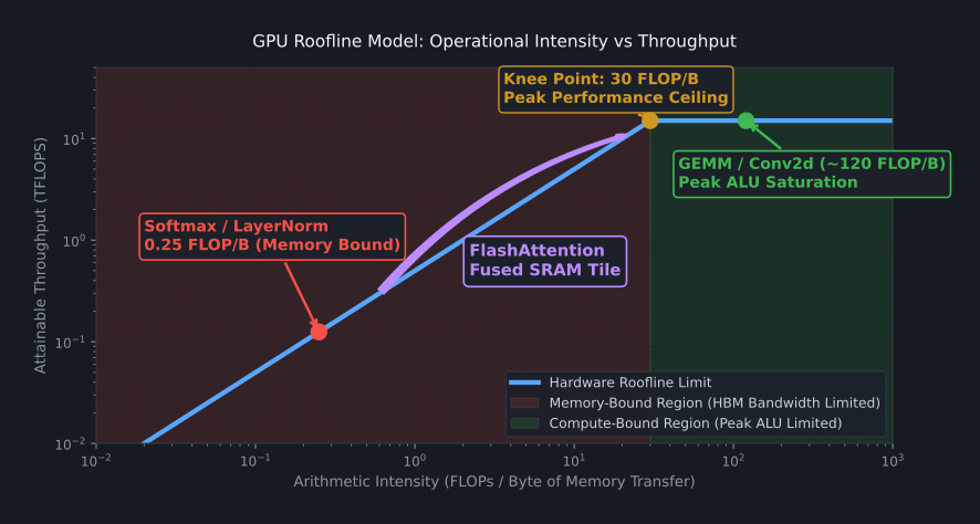
Standard elementwise operations and Softmax have an arithmetic intensity of $\approx 1 \text{ FLOP / Byte}$. They are severely memory-bound. High-throughput GPU programming requires fusing operations so data remains on the fast cutting board (local memory) as long as possible.
3. FlashAttention: Tiling and Online Softmax
Dao et al. (2022) solved the attention memory bottleneck by recognizing that we never need to materialize the $(S \times S)$ matrix in VRAM at all.
FlashAttention computes exact attention by breaking $\mathbf{Q}, \mathbf{K}, \mathbf{V}$ into small blocks that fit entirely inside on-chip local memory (SRAM), fusing the dot product, Softmax, and value reduction into a single kernel pass.
The Challenge: How to Compute Softmax in Chunks?
Standard Softmax requires summing across the entire sequence row to compute the normalization denominator:
$$\text{softmax}(\mathbf{z})_i = \frac{e^{z_i - m}}{\sum_{j=1}^S e^{z_j - m}}, \quad m = \max_{j}(z_j)$$
The Intuitive Dilemma: Grading Tests Through a Mail Slot
Imagine you are an OpenCL compute unit with only 48 KB of local SRAM. You are grading test scores one by one through a narrow mail slot. You want to normalize everyone's score relative to the class maximum $m$.
After grading the first two tests, the highest score you have seen is $4.0$. You divide by your current running sum. Suddenly, test #3 arrives with a score of $5.0$!
Your previous maximum is obsolete. All your old exponential weights are now too large! Do you have to throw away all your work, walk back to the basement VRAM, and re-read the entire sequence from scratch?
Dao et al. (2022) and Milakov & Gimelshein (2018) proved that you do not. You only need a single mathematical lever ($\alpha$) to rescale your previous accumulator in $O(1)$ constant time inside fast GPU registers!
Zero Hidden Premises: Symbol Breakdown
| Symbol | Mathematical Domain | Physical Role in OpenCL Kernel |
|---|---|---|
| $B_r, B_c$ | $\mathbb{N}^+$ | Query block size and Key/Value block size fitting in on-chip local memory (e.g. 64 or 128) |
| $m_{\text{old}}, m_{\text{new}}$ | $\mathbb{R}$ | Running row maximum logit tracked in GPU registers for numerical stability |
| $\ell_{\text{old}}, \ell_{\text{new}}$ | $\mathbb{R}^+$ | Running sum of scaled exponentials (Softmax denominator accumulator) |
| $\alpha = e^{m_{\text{old}} - m_{\text{new}}}$ | $\mathbb{R} \in (0, 1]$ | Rescaling factor that adjusts past accumulations in registers when a new maximum is found |
| $\mathbf{O} \in \mathbb{R}^{d_k}$ | Running unnormalized attention output accumulator kept in fast registers |
The Mathematical Solution: Online Softmax
Suppose we have accumulated the exponential sum over block $A$ with local maximum $m_A$:
$$\ell_A = \sum_{j \in A} e^{z_j - m_A}$$
A new block $B$ arrives with local maximum $m_B$. The combined global maximum is:
$$m_{\text{new}} = \max(m_A, m_B)$$
To adjust the previous exponential terms to the new maximum $m_{\text{new}}$, we rewrite each term using exponent addition rules:
$$e^{z_j - m_{\text{new}}} = e^{(z_j - m_A) + (m_A - m_{\text{new}})} = e^{z_j - m_A} \cdot e^{m_A - m_{\text{new}}} = e^{z_j - m_A} \cdot \alpha$$
Where the scalar correction factor is:
$$\alpha = e^{m_A - m_{\text{new}}} \le 1.0$$
Summing over all elements $j \in A$:
$$\sum_{j \in A} e^{z_j - m_{\text{new}}} = \sum_{j \in A} \left( e^{z_j - m_A} \cdot \alpha \right) = \alpha \sum_{j \in A} e^{z_j - m_A} = \alpha \ell_A$$
We can rescale the entire past accumulated sum by multiplying by $\alpha$ in $O(1)$ constant time, without ever re-reading a single past token from memory!
The Full Online Update Equations
When transitioning from old accumulated statistics to a newly loaded tile $B$:
- Update Running Maximum: $$m_{\text{new}} = \max(m_{\text{old}}, \max_{j \in B}(z_j))$$
- Compute Correction Factor: $$\alpha = e^{m_{\text{old}} - m_{\text{new}}}$$
- Update Running Denominator: $$\ell_{\text{new}} = \alpha \cdot \ell_{\text{old}} + \sum_{j \in B} e^{z_j - m_{\text{new}}}$$
- Update Running Context Vector: $$\mathbf{O}_{\text{new}} = \alpha \cdot \mathbf{O}_{\text{old}} + \sum_{j \in B} e^{z_j - m_{\text{new}}} \mathbf{v}_j$$
At the conclusion of the sequence loop, the final exact attention output is:
$$\mathbf{O}_{\text{final}} = \frac{\mathbf{O}}{\ell}$$
Concrete Worked Numerical Walk-Through: The Chronological State Machine
Let a single query have logits against 4 tokens, arriving in two tiles of size 2 ($d_k = 1$ for visual clarity): - Tile 1: Logits $\mathbf{z}_1 = [2.0, 4.0]$, Values $\mathbf{v}_1 = [10.0, 20.0]$ - Tile 2: Logits $\mathbf{z}_2 = [1.0, 5.0]$, Values $\mathbf{v}_2 = [30.0, 40.0]$
Chronological Register Progression Table
| Timeline Step | Hardware Event | Running Max $m$ | Rescale Factor $\alpha$ | Denominator Acc $\ell$ | Context Acc $\mathbf{O}$ | Physical Interpretation |
|---|---|---|---|---|---|---|
| Step 0: Init | Clear GPU Registers | $-\infty$ | N/A | $0.0000$ | $[0.000]$ | Registers initialized before loop |
| Step 1: Tile 1 | Stream $z_1 = [2, 4], v_1 = [10, 20]$ | $4.0$ | $1.0000$ | $1.1353$ | $[21.353]$ | Partial unnormalized estimate |
| Step 2: Tile 2 | Larger logit ($5.0 > 4.0$) arrives! | $5.0$ | $e^{4-5} \approx 0.3679$ | $1.4360$ | $[48.405]$ | In-place register rescale without VRAM reload |
| Step 3: Final | Single Vector Division $\mathbf{O} / \ell$ | $5.0$ | N/A | $1.4360$ | $[33.708]$ | Mathematically exact output |
Didactic Step-by-Step Mathematical Walk-Through
Tile 1 Arrives in Fast SRAM (Initial Baseline)
GPU loads $\mathbf{z}_1 = [2.0, 4.0]$ and values $\mathbf{v}_1 = [10.0, 20.0]$. We compute the first partial estimates:
Tile 2 Arrives: Larger Logit ($5.0 > 4.0$) & Online Rescaling
New inputs arrive: $\mathbf{z}_2 = [1.0, 5.0]$ and $\mathbf{v}_2 = [30.0, 40.0]$. Because $5.0 > 4.0$, our old baseline $m_1$ is obsolete. Instead of reloading Tile 1 from VRAM, we rescale past registers with scalar $\alpha$:
Final Normalization: Single Vector Division
After all sequence tiles have streamed through SRAM, the final mathematically exact attention output is computed by a single elementwise vector division:
Side-by-Side Proof Against Standard Global Softmax
| Evaluation Method | Softmax Probabilities $\mathbf{A}$ | Output Context Vector $\mathbf{O} = \mathbf{A}\mathbf{V}$ | Peak VRAM Memory Footprint |
|---|---|---|---|
| Standard Offline Softmax | $[0.0347, 0.2562, 0.0127, 0.6964]$ | $0.0347(10) + 0.2562(20) + 0.0127(30) + 0.6964(40) = \mathbf{33.708}$ | Quadratic $O(S^2)$ buffer in VRAM |
| Streaming Online Softmax | Computed on-the-fly in registers | $\mathbf{O}_2 / \ell_2 = 48.4048 / 1.4360 = \mathbf{33.708}$ | Linear $O(S)$ buffer in VRAM |
The numerical results match to 5 decimal places. We achieved exact mathematical equivalence while streaming through memory in small tiles.
Result: Memory consumption drops from $O(S^2)$ to $O(S)$, and wall-clock execution accelerates by $2\times$ to $4\times$.
4. Key-Value (KV) Caching in Autoregressive Generation
When an LLM generates text token by token, the process is autoregressive:
$$\text{Prompt}: \text{"The"} \to \text{"capital"} \to \text{"of"} \to \text{"France"} \to \text{"is"} \to \dots$$
At step $t = 5$, the model computes attention between "is" and all previous tokens.
- In a naive loop, the model would re-project all past tokens through $\mathbf{W}_K$ and $\mathbf{W}_V$ at every step. This scales with quadratic cost $O(T^2)$ for generating $T$ tokens.
- KV-Caching: We project past tokens once, store their key and value vectors in a pre-allocated GPU ring buffer, and only project the single newest token at each step.
Generation cost drops to linear time $O(T)$ per token.
5. Prototypical NetCL Implementation
NetCL implements streaming FlashAttention with local memory tiling and an integrated KVCache in netcl.nn.transformer:
import numpy as np
from netcl.core.device import manager
from netcl.core.tensor import Tensor
from netcl.nn.transformer import KVCache, RotaryAttention

q = manager.default("auto").queue

# 1. Initialize KV-Cache for autoregressive decoding
# Max batch=1, max sequence=2048, heads=4, head_dim=64
kv_cache = KVCache(
    queue=q,
    max_batch_size=1,
    max_seq_len=2048,
    n_kv_heads=4,
    head_dim=64,
)

# 2. Simulate step-by-step token generation
print(f"Allocated KV Cache buffer in GPU memory.")

# Incoming single-token projection at step 0
k_step = Tensor.from_host(q, np.random.randn(1, 1, 4, 64).astype(np.float32))
v_step = Tensor.from_host(q, np.random.randn(1, 1, 4, 64).astype(np.float32))

# Store into cache at position 0
kv_cache.update(k_step, v_step, start_pos=0)
print(f"KV Cache successfully updated for token position 0.")
Related Documentation
- Concepts: Transformer: Architecture documentation for decoder blocks, RoPE, and attention layers.
- Architecture: Tensor Backend: OpenCL memory buffer management and sub-allocations.
- Ops Reference: Attention: GPU kernel primitives for FlashAttention and softmax.
Next Steps in the Curriculum
Now that you have mastered supervised neural architectures for vision and language, what do you do when you have no labels at all?
Proceed to Chapter 9: Clustering & Geometric Machine Learning to explore Voronoi vector quantization, fused distance-argmin execution, and Gaussian Mixtures.