
Calculus, Gradients & Computational Graphs
Calculus, Gradients & Computational Graphs
In Chapter 1: What is Machine Learning?, we established that training a neural network is equivalent to finding the lowest point in a high-dimensional loss landscape.
If you are standing on a foggy mountain and cannot see the bottom, how do you walk down into the valley without guessing blindly?
You feel the slope of the ground under your feet.
This chapter explains calculus from first principles, derives the gradient vector, demystifies the chain rule, and reveals why reverse-mode automatic differentiation (the Tape mechanism) enables deep learning on modern GPUs.
1. Core Intuition: Slopes and Compass Needles
Imagine standing on an undulating loss surface with parameter knobs $\mathbf{w} = (w_1, w_2)$ and an error altitude $\mathcal{L}(\mathbf{w})$.
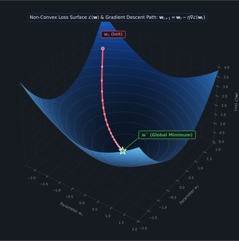
If you nudge a knob by a tiny amount $\Delta w_1 = +0.01$, what happens to the loss? - If the altitude goes up, the slope is positive. To reduce loss, you turn the knob in the opposite direction (decrease $w_1$). - If the altitude goes down, the slope is negative. To reduce loss, you keep turning the knob forward (increase $w_1$).
The gradient vector $\nabla \mathcal{L}(\mathbf{w})$ is simply your compass needle on the 3D hillside: it points directly toward the steepest uphill ascent.
To reach the global valley floor $\mathbf{w}^*$, we take iterative steps in the exact opposite direction: $\mathbf{w}_{t+1} = \mathbf{w}_t - \eta \nabla \mathcal{L}(\mathbf{w}_t)$.
2. Mathematical Formalization: From Slopes to Gradients
The Derivative of a Scalar Function
For a continuous function $f(w)$, the derivative with respect to $w$ is the limit of the rate of change as the step size approaches zero:
$$\frac{df}{dw} = \lim_{h \to 0} \frac{f(w + h) - f(w)}{h}$$
Partial Derivatives in Multi-Parameter Space
In a real neural network, the loss $\mathcal{L}(w_1, w_2, \dots, w_P)$ depends on millions of parameters. A partial derivative $\frac{\partial \mathcal{L}}{\partial w_i}$ measures how the loss changes when you wiggle parameter $w_i$ while holding all other parameters fixed.
The Gradient Vector ($\nabla \mathcal{L}$)
The collection of all partial derivatives assembled into a single vector is the gradient:
$$\nabla_\theta \mathcal{L} = \begin{bmatrix} \frac{\partial \mathcal{L}}{\partial \theta_1} \\ \frac{\partial \mathcal{L}}{\partial \theta_2} \\ \vdots \\ \frac{\partial \mathcal{L}}{\partial \theta_P} \end{bmatrix}$$
Key Geometric Property: - The gradient vector $\nabla \mathcal{L}$ points in the direction of steepest ascent (the fastest way uphill). - The negative gradient $-\nabla \mathcal{L}$ points in the direction of steepest descent (the fastest way downhill).
Zero Hidden Premises: Symbol Breakdown
| Symbol | Mathematical Domain | Physical Role & Hardware Meaning |
|---|---|---|
| $\boldsymbol{\theta}$ | $\mathbb{R}^P$ | Total model parameter vector ($P$ trainable weights and biases in VRAM) |
| $\mathcal{L}$ | $\mathbb{R}$ | Scalar loss output (objective to be minimized) |
| $\nabla_{\boldsymbol{\theta}} \mathcal{L}$ | $\mathbb{R}^P$ | Gradient vector of partial derivatives $\left[ \frac{\partial \mathcal{L}}{\partial \theta_1}, \dots, \frac{\partial \mathcal{L}}{\partial \theta_P} \right]^T$ |
| $\mathbf{J} \in \mathbb{R}^{M \times K}$ | Jacobian Matrix | Matrix of first-order partial derivatives $J_{ij} = \frac{\partial f_i}{\partial x_j}$ for layer $\mathbf{f}: \mathbb{R}^K \to \mathbb{R}^M$ |
| $\mathbf{v}^T \mathbf{J}$ | Vector-Jacobian Product (VJP) | Reverse-mode primitive: projects incoming sensitivity $\mathbf{v} \in \mathbb{R}^M$ back to inputs $\mathbb{R}^K$ |
| $\mathbf{J} \mathbf{v}$ | Jacobian-Vector Product (JVP) | Forward-mode primitive: pushes directional perturbation forward |
3. The Chain Rule: Composing Operations
Deep neural networks do not compute the loss in a single monolithic formula. They chain operations in sequence:
$$\mathbf{x} \xrightarrow{\quad f_1 \quad} \mathbf{h}_1 \xrightarrow{\quad f_2 \quad} \mathbf{h}_2 \xrightarrow{\quad f_3 \quad} \hat{\mathbf{y}} \xrightarrow{\quad \mathcal{L} \quad} \text{Loss}$$
To find how an early parameter $w$ inside $f_1$ affects the final loss, we apply the Chain Rule of Calculus:
$$\frac{\partial \mathcal{L}}{\partial w} = \frac{\partial \mathcal{L}}{\partial \hat{\mathbf{y}}} \cdot \frac{\partial \hat{\mathbf{y}}}{\partial \mathbf{h}_2} \cdot \frac{\partial \mathbf{h}_2}{\partial \mathbf{h}_1} \cdot \frac{\partial \mathbf{h}_1}{\partial w}$$
Every layer receives a sensitivity signal from the layer ahead of it, multiplies that signal by its own local derivative, and passes the product backward to the preceding layer.
Concrete Worked Numerical Step: A 2-Layer Computation
Let input $x = 2.0$, initial weight $w = 3.0$, bias $b = 1.0$, and ground-truth target $y = 10.0$.
Phase 1: Forward Pass
The signals propagate from input to scalar loss:
-
Affine Linear Combination: $$z = w \cdot x + b = (3.0 \cdot 2.0) + 1.0 = 7.0$$
-
Activation Function ($\text{ReLU}$): $$a = \text{ReLU}(z) = \max(0, 7.0) = 7.0$$
-
Mean Squared Error Loss: $$\mathcal{L} = (a - y)^2 = (7.0 - 10.0)^2 = (-3.0)^2 = 9.0$$
Phase 2: Reverse Pass (Step-by-Step Backpropagation)
The sensitivity signal traverses backward from the scalar loss to each trainable parameter via the chain rule:
-
Seed the gradient at the scalar loss root: $$\frac{\partial \mathcal{L}}{\partial \mathcal{L}} = 1.0$$
-
Loss gradient with respect to activation $a$: $$\frac{\partial \mathcal{L}}{\partial a} = \frac{\partial}{\partial a} (a - y)^2 = 2(a - y) = 2(7.0 - 10.0) = -6.0$$
-
Local gradient through the ReLU non-linearity: $$\frac{\partial \mathcal{L}}{\partial z} = \frac{\partial \mathcal{L}}{\partial a} \cdot \frac{da}{dz} = (-6.0) \cdot \mathbb{I}_{z > 0} = (-6.0) \cdot 1.0 = -6.0$$
-
Parameter gradient for weight $w$: $$\frac{\partial \mathcal{L}}{\partial w} = \frac{\partial \mathcal{L}}{\partial z} \cdot \frac{\partial z}{\partial w} = (-6.0) \cdot x = (-6.0) \cdot 2.0 = -12.0$$
-
Parameter gradient for bias $b$: $$\frac{\partial \mathcal{L}}{\partial b} = \frac{\partial \mathcal{L}}{\partial z} \cdot \frac{\partial z}{\partial b} = (-6.0) \cdot 1.0 = -6.0$$
Phase 3: Parameter Update & Verification
With learning rate $\eta = 0.05$, gradient descent steps update each parameter:
$$w \leftarrow w - \eta \frac{\partial \mathcal{L}}{\partial w} = 3.0 - (0.05 \cdot (-12.0)) = 3.0 + 0.60 = 3.60$$
$$b \leftarrow b - \eta \frac{\partial \mathcal{L}}{\partial b} = 1.0 - (0.05 \cdot (-6.0)) = 1.0 + 0.30 = 1.30$$
Testing the updated model on the same input:
$$z_{\text{new}} = (3.60 \cdot 2.0) + 1.30 = 8.50 \implies a_{\text{new}} = 8.50$$
$$\mathcal{L}_{\text{new}} = (8.50 - 10.0)^2 = (-1.50)^2 = 2.25$$
The single gradient descent step reduced the objective loss from $9.00$ to $2.25$ (a 75% error reduction in one iteration).
4. Why Backpropagation? Forward vs. Reverse-Mode Autograd
There are two distinct ways to evaluate the chain rule across a computational graph:
| Feature | Forward-Mode Automatic Differentiation | Reverse-Mode Autodiff (Backpropagation) |
|---|---|---|
| Traversal Direction | Inputs $\to$ Outputs | Outputs $\to$ Inputs |
| Core Operator | Jacobian-Vector Product (JVP): $\mathbf{J}\mathbf{v}$ | Vector-Jacobian Product (VJP): $\mathbf{v}^T \mathbf{J}$ |
| Passes Needed | $O(P)$ forward passes (1 per parameter) | $O(1)$ single reverse pass (independent of $P$) |
| Optimal Use Case | Few inputs ($P \ll M$), e.g. 3D physics raytracing | Many inputs, scalar loss ($P \gg M = 1$), e.g. Deep Learning |
| Memory Requirement | Minimal (no intermediate activations saved) | Must retain forward activations on the Tape until backward pass completes |
Because deep learning models have 1 scalar output (loss $\mathcal{L} \in \mathbb{R}$) but millions of input parameters ($\boldsymbol{\theta} \in \mathbb{R}^P$), reverse-mode automatic differentiation is mathematically optimal. If we used forward-mode on a 7-billion parameter model, training would require 7 billion forward passes per mini-batch! Reverse-mode computes all 7 billion gradients in exactly one backward pass.
5. The Computational Graph & The Tape Mechanism
How does netcl implement reverse-mode automatic differentiation?
Instead of building a static graph upfront (like older frameworks), netcl uses a dynamic execution tape:
Tape records: matmul_backward"] H -->|"ag.add"| Logits["Logits Node
Tape records: add_backward"] Logits -->|"ag.cross_entropy"| Loss["Scalar Loss Node
Tape records: cross_entropy_backward"] end subgraph Reverse["Reverse Traversal: tape.backward()"] Loss ==>|"Seed dL/dL = 1.0"| Backward["Unwind Tape Stack in Reverse"] Backward -->|"Dispatch OpenCL Kernels"| Grad["Leaf Gradients: W.grad, b.grad"] end
- Passive Buffer vs. Active Node: A raw
netcl.Tensoris just GPU memory (cl_mem). Wrapping it withag.tensor(t)turns it into aNodecontaining graph connectivity. - Tape Recording: During
with ag.Tape() as tape:, every operation executed on nodes automatically appends an entry to the tape's internal stack. The tape remembers the input nodes, output nodes, and the corresponding gradient function. - Reverse Topological Traversal: When you call
tape.backward(loss), netcl seeds the loss gradient $\frac{\partial \mathcal{L}}{\partial \mathcal{L}} = 1.0$, unwinds the recorded tape in reverse chronological order, and executes the backward OpenCL kernels. - Gradient Accumulation: Gradients are written directly into the
.gradattribute of each leaf parameter tensor.
6. Prototypical NetCL Implementation
Here is a self-contained demonstration showing the complete autograd lifecycle:
import numpy as np
import netcl.autograd as ag
from netcl.core.device import manager
from netcl.core.tensor import Tensor

q = manager.default("auto").queue

# 1. Create leaf parameters on GPU device
w_raw = Tensor.from_host(q, np.array([3.0], dtype=np.float32))
b_raw = Tensor.from_host(q, np.array([2.0], dtype=np.float32))
x_raw = Tensor.from_host(q, np.array([4.0], dtype=np.float32))

# 2. Record graph on the Tape: y = (w * x + b)^2
with ag.Tape() as tape:
    # Wrap into graph nodes
    w = ag.tensor(w_raw)
    b = ag.tensor(b_raw)
    x = ag.tensor(x_raw)

    linear = ag.add(ag.mul(w, x), b)   # 3 * 4 + 2 = 14
    loss = ag.mul(linear, linear)      # 14^2 = 196

print(f"Forward Result: {loss.value.to_host()[0]}")

# 3. Trigger reverse-mode automatic differentiation
tape.backward(loss)

# Mathematical verification:
# d(loss)/dw = d(linear^2)/d(linear) * d(linear)/dw = 2 * 14 * x = 28 * 4 = 112
print("Computed d(loss)/dw:", w.grad.to_host()[0])
# d(loss)/db = 2 * 14 * 1 = 28
print("Computed d(loss)/db:", b.grad.to_host()[0])

assert np.isclose(w.grad.to_host()[0], 112.0)
assert np.isclose(b.grad.to_host()[0], 28.0)
print("Autograd derivatives match exact analytical calculus.")
Related Documentation
- Tutorial: Understanding Autograd: Build custom forward-backward operations and explore node wrapping in depth.
- Autograd API Reference: Complete signature listing for
Tape,Node,no_grad, and autograd primitives. - Concepts: Tape: Architectural guide to topological sorting and kernel dispatch.
Next Steps in the Curriculum
Now that we can compute exact gradients $\nabla_\theta \mathcal{L}$ for millions of parameters, how do we use these gradients to update our weights effectively without oscillating or getting stuck in saddle points?
Proceed to Chapter 3: Neural Building Blocks to learn why single layers collapse and why non-linear activations enable deep representations.